Preamble

Memory Layouts

Before getting into the nitty-gritty, we should remind ourselves how our programs are represented in memory, and how our CPU executes them. The stack and the heap are two components emphasised in the memory layout of a program in COMP1511. The heap consists of memory that is mostly accessed by the programmer through functions such as malloc, and hence it falls upon the programmer to relinquish that memory as well. The stack, on the other hand, is governed by the program's calling convention and is managed automatically as functions are invoked and return, as well as for storing local variables and other information associated with active function calls.
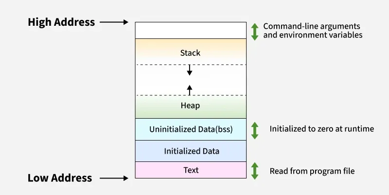
Typical process memory layout from low to high addresses: text, initialized data, uninitialized data (BSS), a heap growing upward, a stack growing downward, and command-line arguments and environment variables
Other than the stack and the heap, there also exist the text/code segment and the data segment(s). The text segment stores the executable machine instructions produced from our source code during compilation. Following this are the data regions, which contain longer lived program data such as global variables, static variables, and string literals. The precise addresses and arrangements of these regions is contingent on the executable format and environment, but it is generally understood that the text and data segments at lower addresses, the heap above them, and the stack near the upper end of the address space.

The stack becomes especially important once we begin working with functions; the more detailed discussion of stack frames and recursion is in MIPS Functions.

The CPU

Storing a program in memory is, of course, insufficient to make it execute. The responsibility for carrying out the program’s instructions falls to the CPU. The CPU does not directly understand C, Python, or even the textual representation of MIPS assembly; it ultimately operates on machine instructions, encoded as binary values and stored within the program’s text segment.

Before understanding how the CPU executes or interprets the instructions we write, however, we must first look at the components the CPU uses to performs its operations.

Registers

Often times we need to do simple operations such as writing or reading a stored value, and perform some computations on those values. However, accessing a value stored in RAM is relatively slow compared to the speed at which a modern CPU operates. A typical access to main memory may take somewhere on the order of ~50–100 ns due to the work involved in accessing and transferring that data back to the processor. Whilst this may seem to be fast, a CPU with a speed of 5 GHz has a clock cycle of only 0.2ns. This means that a 100 ns memory access corresponds to roughly 500 CPU cycles. Waiting directly on RAM for every operation would therefore leave the processor idle for a considerable amount of time. Instead, most CPU architectures perform their actual operations using a much smaller amount of storage found within the processor itself, the registers.
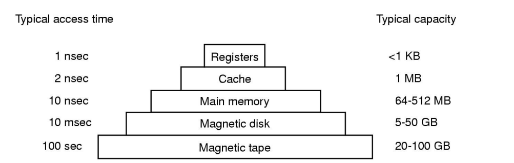
Memory hierarchy pyramid showing registers as fastest and smallest, followed by cache, main memory, magnetic disk, and magnetic tape as slower and larger
Since registers form part of the CPU rather than the RAM, they can be accessed considerably faster than values stored in memory. However, we trade off this speed for space. Compared to memory, we have a relatively small number of registers available. As a consequence, values stored in memory generally need to be loaded into registers before the CPU can perform computations on them. Once the CPU has finished operating on a value, it can later be stored back into memory if necessary.

There are, however, varying types of registers. Some registers are used primarily to hold data for computations, while others have specialised roles in controlling the processor. Registers may also serve different purposes, there can exist registers that exist solely for storing floating-point numbers (FPRs), and there can be registers that hold read-only constants such as zero. Registers are normally measured by the number of bits they can hold, for example, an 8-bit register, 32-bit register, 64-bit register, 128-bit register, or more. This determines the range of bit patterns that can be represented in that register at any one time. The width of the general-purpose registers is often closely related to the architecture itself, which is why we commonly describe architectures as 32-bit or 64-bit.

Of these specialised registers, one is especially important for understanding how these programs run, the Program Counter. If the CPU executes the given instructions, it needs a way track and know which instruction to go to next (as it isn't always one line after another).

The Life of a CPU

At a simplified level, the CPU continually performs a cycle of fetching, decoding and executing. The CPU keeps track of its current position in the program using a special register known as the Program Counter (PC). Usually, after one instruction executes, the PC advances to the following instruction:

int program_counter = START_ADDRESS; 
while (1) { 
	// Fetch an instruction from memory 
	int instruction = memory[program_counter]; 
	// Move to the next instruction 
	program_counter++; 
	// Execute the next instruction 
	execute(instruction, &program_counter); 
						// ^ note: some instructions may 
						// modify the program counter 
}

The Program Counter holds the memory address of the instruction that the CPU is currently about to execute. Rather than the CPU somehow “knowing” where it is in a program, its location is tracked and stored as part of the processor's state. The PC isn't always sequential however, it does not always move in a fixed manner as control-flow instructions still exist; otherwise logic such as if statements and while loops would not be possible.

A question arises however, what constitutes as an "instruction"? Is an instruction simply a one-line statement similar to calling printf()?

Instructions

Individual instructions understood by the CPU are extremely primitive, it is rather a large combination of these instructions that lets us create more sophisticated behaviour.

CPU instructions can broadly include:

Computations: arithmetic and bitwise operations such as add, subtract, multiply, divide, XOR
Load/store: Load data from memory into CPU registers, and store data from registers back into memory
Branching: jumping between instructions rather than sequentially processing (this is what lets us use logic such as if statements and while loops)
System calls: requesting the OS to perform an action (i.e. read from a file)

These instructions are not universal, however. Different processor architectures may provide different registers, instructions and encodings. This is part of the reason why MIPS (most likely) cannot be run on your laptop.

Instruction Set Architectures

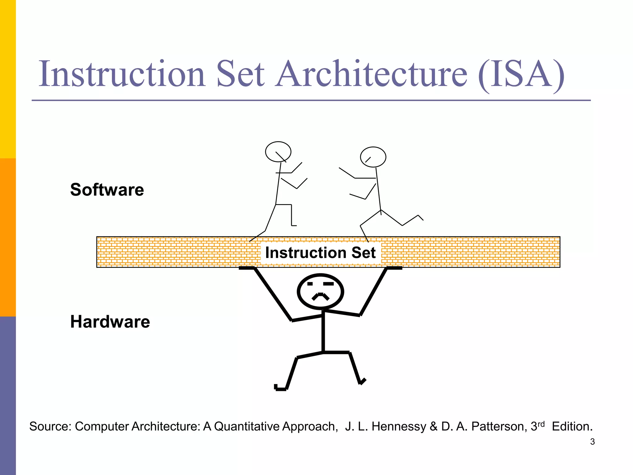
As mentioned prior, registers can differ in width and purpose, and processors themselves may be designed around different sets of instructions, registers, and conventions. These specifications are known as Instruction Set Architectures (ISAs) and can include x86-64, ARM64, RISC-V, and MIPS. An ISA can essentially be thought of as the "contract" between a computer's software and hardware. It determines the instructions that software may ask the CPU to perform, the registers available to those instructions, and how those instructions are represented and behave. Two processors implementing different ISAs may therefore expose completely different instructions even if, at a higher level, both are capable of accomplishing the same tasks.

MIPS therefore is not simply another programming language that we can freely switch to in the same way we might switch between, say, Python and C. While higher-level languages such as C can be compiled into machine instructions for many different target architectures, MIPS assembly is specifically tied to the MIPS instruction set. It is worth noting, however, that translation and emulation techniques do exist which allow MIPS programs to be run on machines using a different host architecture (see: Running MIPS). In essence, MIPS assembly corresponds specifically to the MIPS architecture.
Instruction set architecture shown as the interface between software above and hardware below
Furthermore, the term "assembly language" does not denote one singular language, similar to how the term "high level language" does not entail one specific language. Assembly is a class of low-level languages, and MIPS assembly is part of that class. This means that MIPS and MIPS assembly are distinct terms: the former refers to an ISA, while the latter refers to the assembly language used to represent instructions from that architecture. COMP1521 focuses specifically on MIPS because it provides a comparatively simple instruction set while still exposing the fundamental ideas found in other architectures. MIPS has also influenced other ISAs, and understanding it provides a useful foundation for learning architectures such as ARM and RISC-V.

Assembly language, however, is still not the final layer before the CPU executes the program. Although assembly gives us a human-readable representation of the processor’s instructions, the CPU itself ultimately operates on those instructions in a form abstracted one layer less.

Machine Code

The CPU cannot understand the textual instructions written in languages such as C, and even when descending a layer further, it still cannot directly execute the MIPS assembly that we write. These instructions are instead represented as patterns of bits (1s and 0s) known as machine code.

Each instruction in a CPU's ISA has a defined binary encoding, which is why MIPS machine instructions cannot simply be executed by an x86-64 processor: the two architectures interpret instruction encodings according to different ISAs. In MIPS32, instructions are normally encoded as 32-bit machine instructions, with different groups of bits representing information such as the operation to perform, the registers involved, and any constant values used by the instruction.

This is better depicted by the following image:
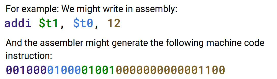
MIPS ADDI instruction encoding showing the opcode, source register, destination register, and immediate fields
Here, addi $t1, $t0, 12 simply mean $t1 = $t0 + 12. However, the processor does not execute the text addi $t1, $t0, 12. A special tool known as the assembler translates this assembly instruction into its corresponding machine-code representation. The first six bits, 001000, identify the instruction as addi. The following fields identify the source register $t0, the destination register $t1, and the immediate value 12. The official MIPS32 encoding for ADDI is 001000 | rs | rt | immediate, using fields of 6, 5, 5, and 16 bits respectively.

Therefore, assembly language is a human-readable representation of machine instructions. We write symbolic names such as addi, $t0, and $t1, while the CPU ultimately fetches and executes their binary machine-code encodings. So then, why does compilation from a C program seem so easy?

Building

When we normally compile a C program:

BASH

gcc hello.c -o hello

It can be perceived as one step, the black box known as "compilation" occurs and we now have our executable. However, compilers such as GCC & Clang (and by extension DCC) conceal several intermediate stages. GCC acts as a compiler driver, it does not act as one tool but rather manages many tools that are required to convert your code into an executable format.

A compiler roughly follows these steps:

flowchart LR
    A["C Source Code<br/>hello.c"] --> B["Preprocessor"]
    B --> C["Preprocessed C"]
    C --> D["Compiler"]
    D --> E["Assembly<br/>hello.s"]
    E --> F["Assembler"]
    F --> G["Object File<br/>hello.o"]
    G --> H["Linker"]
    H --> I["Executable<br/>hello"]

These intermediate files, such as assembly code or object code, do not necessarily have to be written to disk every time we run gcc; the compiler driver can invoke each stage for us. Nevertheless, separating the process conceptually is important because each stage performs a different job and produces a different form of the program.

The Preprocessor

Before converting the code into assembly code, we must first "process" the code, we have to resolve the #includes and #defines, and conditional compilation directives such as #if. These directives are processed before the compiler properly begins translating the program.

When we write

#include <stdio.h>

the required declarations from the header must be made available as part of the source presented to the later compilation stages. Similarly, macros created using #define are expanded by the preprocessor before compilation occurs. The result is therefore still C source code, but most likely expanded by ALOT.

We can ask GCC to stop after this step with:

BASH

gcc -E hello.c -o hello.i

producing a preprocessed source file conventionally given the .i extension. Although this file may be considerably larger and uglier than the original program we wrote, it has still not been converted into instructions understood by the CPU. This is where the compiler takes action.

The Compiler

The compiler takes the preprocessed C program and translates it into instructions for a particular target architecture. This is where the higher-level constructs we write in C, such as expressions, loops, conditionals and function calls, begin to be transformed into much simpler operations available in the target ISA.

The compiler also performs much more than blindly translating each line of C one-for-one. A single C statement may require several assembly instructions, while other pieces of code may be rearranged or eliminated entirely through optimisation. Ultimately, however, the output can be represented as assembly code belonging to the architecture being targeted.
For example, GCC allows us to stop after this stage using:

BASH

gcc -S hello.c

which produces an assembly source file such as hello.s. This is the intermediate stage normally hidden when we simply run gcc hello.c -o hello.

At this point, however, we still only possess the human-readable representation of those CPU instructions. As established previously, the CPU cannot directly execute assembly source code. We must therefore descend one layer further.

The Assembler

Since the CPU can't understand assembly code, we need a tool that converts that human-readable code into machine-readable code. This is called the assembler.

The assembler reads instructions such as:

MIPS

addi $t1, $t0, 12

and encodes them into the corresponding machine instructions defined by the target ISA. It also processes labels and assembler directives, keeping track of information that may be needed later when the program is finally put together.

The output from this stage is normally an object file. For example, a source file such as:

BASH

hello.s

may be assembled into:

BASH

hello.o

The .o file now contains actual machine code, but somewhat confusingly, this still does not necessarily mean that we have a complete program which can simply be executed.

Object Files

An object file contains the machine code and data produced from one unit of compilation, alongside additional information required to eventually construct the complete executable. This can include information about symbols, sections of the program, and locations whose final addresses are not yet known.

This is necessary because programs rarely exist as a single completely isolated source file. Suppose main.c contains a call to a function defined in another file:

int result = calculate();

The compiler can generate the instructions required to call calculate, but while compiling main.c by itself, it may not yet know where the machine code for calculate will ultimately reside in the finished program. Likewise, calls to functions from libraries such as printf refer to code which was not written in our own source file at all.

An object file can therefore contain machine instructions whilst still having references which need to be connected to code or data elsewhere. Before the program can become a complete executable, these pieces must be brought together. This is the job of the linker.

The Linker

The linker takes one or more object files, together with any required libraries, and combines them into the final executable program. During this process it resolves references between the different pieces of the program, determining where functions and data ultimately reside and connecting references to their appropriate definitions.

For example, if we had:

main.o
math.o

where main.o contains a call to a function defined inside math.o, the linker can resolve that reference when constructing the final executable. References to library code are similarly handled according to the libraries and linking environment being used.

This is an important distinction between an object file and an executable. Both may contain machine code, but an object file is generally still an intermediate component intended to be linked with other components, whereas an executable has been arranged into the format required for the operating system to load and run it.

Thus, our original source has now travelled roughly through:

flowchart TD
    A["hello.c"] -->|Preprocessing| B["Preprocessed C"]
    B -->|Compilation| C["hello.s"]
    C -->|Assembly| D["hello.o"]
    D -->|Linking| E["hello"]

At last, we have an executable file containing machine instructions for our target architecture. However, simply having an executable sitting somewhere on our disk is no more sufficient to make it run than having our original C file was.

Loading and Running a Program

An executable is ultimately still just a file stored on some form of persistent storage. Before the CPU can begin executing its instructions, the information contained within that file must be placed into the program's address space in memory.

When we run a program, the operating system's program-loading machinery reads the executable and maps or loads its required components into the appropriate regions of memory. The executable's machine instructions become available in the program's text/code region, while its data contributes to the appropriate data regions. The process is also given the runtime state required for execution, including a stack, with other facilities such as dynamically loaded libraries being prepared where necessary.

This brings us back to the memory layout with which we began. The text segment that we earlier described as containing executable machine instructions did not somehow begin with those instructions already inside it; they originated from our source code, passed through the compilation toolchain, were stored within an executable file, and were then made available in memory when that program was run.

Execution must also begin somewhere. An executable specifies an entry point, which determines where execution initially begins. For a normal C program this is not necessarily main() itself; startup code runs first and eventually invokes our main function. Once the initial processor state has been established, the Program Counter is directed to the appropriate starting instruction.

From there, the mechanism should now be familiar. The CPU fetches the machine instruction at the address indicated by the Program Counter, decodes it, executes it, and continues through the program according to the instructions it encounters.

Our journey from the source code we write to the instructions actually carried out by the processor can therefore be summarised as:

flowchart TB
    A["C Source"] --> B["Preprocessor"]
    B --> C["Compiler"]
    C --> D["Assembly"]
    D --> E["Assembler"]
    E --> F["Object Files"]
    F --> G["Linker"]
    G --> H["Executable"]
    H --> I["Loaded into Memory"]
    I --> J["CPU Executes Machine Code"]