03. Analysis of Algorithms

Measure Growth, Not Just Seconds#

A faster computer changes how quickly work is performed. A better algorithm can change how much work is required. To compare algorithms, define the input size, the operation being measured and a cost model. For a scan of an integer array, n is its length and comparing two integers is constant-time. For strings, comparing two keys may inspect many characters and must not silently be counted as constant work.

The lecture's travelling-salesperson story is a warning about growth, not a claim that every solution must try every tour. If we naively enumerate orders of n distinct cities, there are up to n! orders before we even price their edges. Increasing n from 10 to 11 multiplies that candidate count by 11. Hardware that performs a fixed number of extra operations per second cannot compensate for repeated factorial multiplication as n grows. Better algorithms, approximation or constraints may change the task, but analysing the stated algorithm comes first.

Empirical analysis implements an algorithm and measures it. Results depend on input, compiler, machine load and hardware; small jobs can fall below timer resolution. Theoretical analysis expresses work as a function of input size, usually counting representative operations. The two methods complement one another: theory explains scaling, measurements reveal constants and practical effects.

Best, Worst, Average, Expected and Amortised#

For a fixed size n, the best case is the cheapest valid input and the worst case the most expensive. An average-case result averages over a stated input distribution, such as uniformly random permutations. An expected result can average over the algorithm's own random choices, as in randomised pivot selection. An amortised result bounds the total work across a sequence of operations and divides by the number of operations; it need not involve randomness.

Linear search illustrates the distinction. A successful search for the first entry uses one comparison; an absent key uses n. If a successful target is equally likely to occupy any of the n positions, expected comparisons are (1+2+...+n)/n = (n+1)/2. That distribution says nothing about how often targets are absent. A different workload can produce a different average while leaving the worst case unchanged.

Practice. A dynamic array occasionally copies all its entries when it doubles capacity. Does a constant amortised append bound mean every append is constant-time?

From Primitive Counts to Asymptotic Bounds#

An asymptotic statement describes behaviour as size grows. Constant factors and lower-order terms stop controlling the shape: for n² + 4n + 10, dividing by n² gives 1 + 4/n + 10/n², which approaches 1.

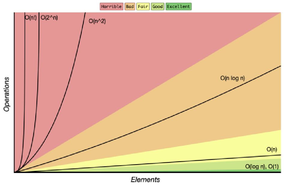
Read the horizontal axis as input size and the vertical axis as operation count. The chart explains why exponential or factorial work quickly overwhelms hardware improvements. Its colours are an illustration, not universal practical cutoffs: a quadratic algorithm can be perfectly adequate for a small bounded input.

Big-Oh, written $O(g(n))$, is an eventual upper bound up to a constant factor: there are positive constants $c,n_0$ such that $f(n)\leq c g(n)$ for all $n\geq n_0$. Big-Omega, $\Omega(g(n))$, is a corresponding lower bound. Big-Theta, $\Theta(g(n))$, means both bounds hold, giving a tight growth class. The slides chiefly use Big-Oh; Theta is useful when the mechanism establishes both sides.

An algorithm doing exactly n comparisons is O(n), but also O(n²). The tight statement is Θ(n). Big-Oh is not inherently “worst case”: you can give an upper bound for best-case or expected work too. Always state which function you are bounding.

Pseudocode and the Measured Operation#

Pseudocode states an algorithm's steps without committing to a programming language's syntax or a particular machine. It should still name the input, output, preconditions and stopping rule. For example, the lecture search contract is “return the first index whose item equals value, otherwise -1”:

linearSearch(A, value):
    for i from 0 to length(A)-1:
        if A[i] == value: return i
    return -1

A worst-case trace on an absent value checks each of the n entries; a best-case trace checks only the first. If A[i] == value compares fixed-width integers, each check is constant-time. If values are strings of length up to L, one equality check can inspect L characters and a faithful worst-case bound becomes O(nL). Naming the primitive is what makes a cost derivation defensible.

Practice. For findSmallest on a nonempty array of n integers, how many value comparisons are necessary in the usual one-pass scan? Why is the best-case count the same?

A Small Exact Count#

For an unsuccessful linear search, the deck's chosen primitive model counts loop initialisation once, loop-condition tests n+1 times, increments n times, indexed comparisons 2n units and the final return once. This gives 4n+3. Another sensible machine-level accounting gives a different constant, but both lead to linear growth.

The following original illustration separates loop-control counts from comparisons:

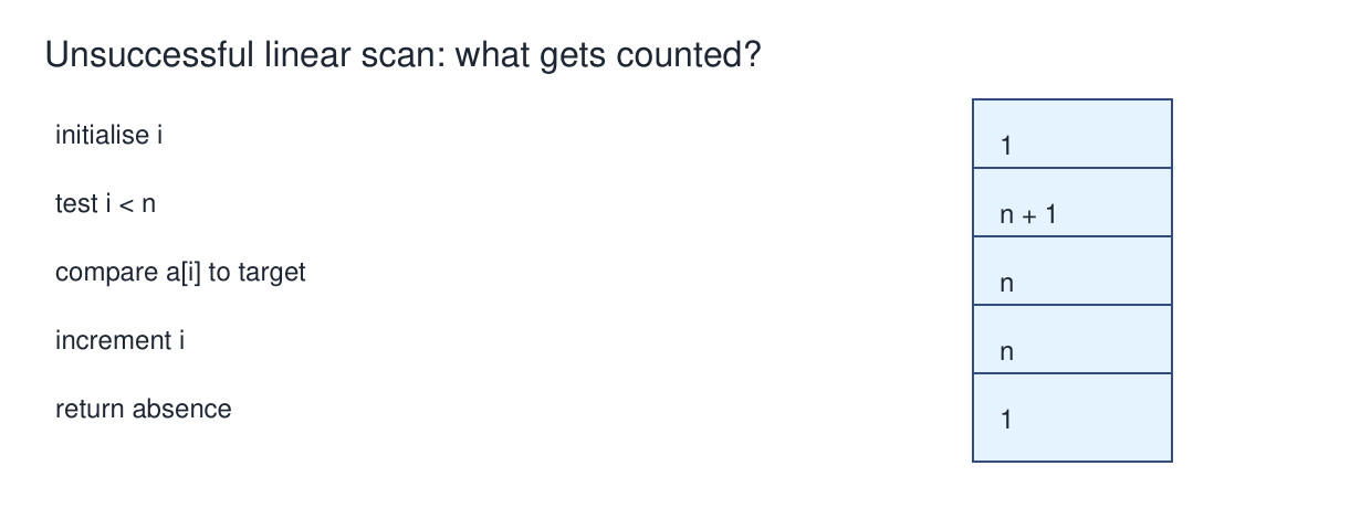
The extra loop check occurs after the final increment, when i == n and the condition fails. We do not need to count every CPU instruction to establish a linear bound. We do need to know whether the loop body hides another scan or a costly string operation.

Practice. Simplify 17n, n³+67n²+144n+12, n log n+log n+12, and 100000+n²+14n to tight growth classes.

Derive Loop Costs#

Sequential and Independent Nested Loops#

Two successive full scans of one array cost n+n, hence Θ(n). Two independent nested loops of lengths n and m execute their body nm times, hence Θ(nm) if that body is constant-time. Three full loops nested with length n each produce n³ iterations.

For the deck's two-array equality example, every item in A is compared with every item in B: Θ(nm). If duplicates exist, that code counts equal pairs, not necessarily distinct common values. For A=[2,2] and B=[2,2,2], it counts six equal pairs, not one shared distinct value. Understanding the output specification comes before deriving a complexity.

Triangular Loops#

for (int i = 0; i < n; i++) {
    for (int j = i + 1; j < n; j++) {
        // compare a[i] with a[j]
    }
}

The inner lengths are n-1,n-2,...,1,0. Thus the total is

$$\sum_{k=1}^{n-1} k=\frac{n(n-1)}2=\Theta(n^2).$$

One way to see the formula is to pair the sum with its reversal: every one of the n-1 pairs adds to n, then divide by two. Early return can reduce some inputs' work. A duplicate finder has a constant-time best case if its first comparison succeeds, but a quadratic worst case when all keys are distinct.

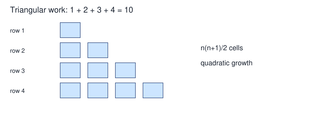
Each row is one outer-loop iteration. Rows grow instead of all having maximum width, but the triangle still occupies a constant fraction of a square. That is why the factor one-half changes an exact count without changing quadratic growth.

Practice. The inner loop runs j=1 through i, with outer i=1 through n. Derive the count. What if the inner loop always runs only five times?

Doubling and Cumulative Progress#

For i = 1; i <= n; i *= 2, the values are 1,2,4,...,2^k. The last exponent satisfies 2^k <= n, so there are floor(log₂ n)+1 iterations. Assume the loop control uses a type/range that avoids overflow. More generally any fixed multiplicative growth factor greater than one gives logarithmic iterations.

A logarithm reverses exponentiation: $\log_b n=x$ means $b^x=n$. For example, $\log_2 8=3$ because $2^3=8$. For a fixed base $b>1$, the change-of-base identity is $\log_b n=\log_2 n/\log_2 b$. Its denominator is a constant, so logarithms with different fixed bases have the same asymptotic growth. This is why complexity notation usually writes simply log n.

Now consider the lecture's less obvious loop:

int p = 0;
for (int i = 1; p <= n; i++) {
    p = p + i;
}

After k iterations, p=1+2+...+k=k(k+1)/2. It stops at the smallest k with k(k+1)/2 > n, so k=Θ(√n), under the no-overflow assumption. Looking only at i++ would miss that the stopping condition depends on cumulative progress.

Practice. For n=10, list p after every iteration and state the first failing condition.

Recurrences Describe Recursive Work#

A recurrence relates the cost on one input to costs on smaller inputs plus local work. It does not automatically solve itself: unpack what the calls do.

For list sum, $T(n)=T(n-1)+c$. Repeated substitution gives $T(n)=T(0)+cn$, hence linear. For binary search, $T(n)=T(\lfloor n/2\rfloor)+c$; after k calls the remaining size is about n/2^k. Reaching one takes logarithmically many levels.

For merge sort, $T(n)=2T(n/2)+cn$ for convenient power-of-two sizes. Level zero processes n elements, level one has two subproblems of n/2 each, and level two has four of n/4 each. Total local work per level stays linear, with logarithmically many levels. Therefore total work is Θ(n log n). Non-power-of-two sizes change rounding, not the class.

By contrast, splitting off one pivot at a time gives $T(n)=T(n-1)+cn$. Expanding sums n+(n-1)+...+1, producing quadratic time. Recursion is not synonymous with logarithmic work.

Practice. A routine makes two recursive calls on n-1 and constant local work. How does that differ from list sum?

Storage, Multiple Sizes and Preprocessing#

An in-place scan needs a few variables, so constant auxiliary space; the input array itself still occupies linear storage. Merge sort has a linear temporary buffer and logarithmic recursive depth. A matrix graph stores V² possible connections even if only a few edges exist; a list graph stores vertices plus actual edges, Θ(V+E). These variables must remain separate unless the problem explicitly relates them.

The slides ask whether searching can be even faster than binary search. A hash table can give expected constant-time lookup under suitable hashing and load assumptions, but building and storing that index costs time and space, and its worst-case lookup need not be constant. There is no contradiction with linear search on a raw unordered array: the faster query is possible because the representation and preprocessing changed. Hash Tables derives those conditions.

Sorting once before many searches can be worthwhile: if sorting costs Θ(n log n) and each binary search costs O(log n), then q queries take O(n log n + q log n) overall. Repeated linear searches cost O(qn). Reporting only the binary-search term hides the preprocessing cost; reporting only sorting hides the workload benefit.

For O(n+m), the two variables can grow independently. You can equivalently write O(max(n,m)) up to a factor of two, but not casually replace them by O(n) if m can be much larger. “Constant-time hashing” similarly requires explicit load and key-cost assumptions, developed in Hash Tables.

More exam-style practice#

Work each prompt before opening its answer. State the invariant or cost assumption that makes your reasoning valid.

Question 1. Count the iterations of for (i = 1; i < n; i *= 2) for n = 9, then give its asymptotic bound.

Question 2. An outer loop runs i = 0..n-1; its inner loop runs j = 0..i. Give the exact number of body executions and the bound.

Question 3. A data structure doubles its capacity when full. Why can a single append cost Θ(n) while a sequence of n appends costs Θ(n) total?