10. Balancing Binary Search Trees
The ordinary BST search rule stays correct even when a tree becomes a chain. Correctness alone therefore does not give the performance we want. Recall from 09. Binary Search Trees that one search costs , where counts edges on a longest root-to-leaf path. Balancing is about controlling that height while retaining the same sorted keys.
We need two ideas: a precise measure of balance, and small changes that preserve BST ordering. Rotations provide those changes. Partitioning combines them to move a chosen sorted position to the root. From there we can either rebuild the whole shape or make cheaper local adjustments.
Two definitions of balance#
The size of a subtree is its number of stored nodes. A size-balanced tree satisfies
at every node. A height-balanced tree satisfies
at every node, with empty height and leaf height 0. These are properties of all rooted subtrees, not just the overall root. “The tree looks roughly symmetrical” is not a definition.
The lecture example rooted at 4 has left subtree rooted at 2 with leaves 1 and 3, and right leaf 5. Blue labels count subtree nodes; red labels give heights. At root 4, left size 3 versus right size 1 differs by two, but left height 1 versus right height 0 differs by only one.
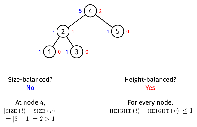
It is height-balanced but not size-balanced. Height balance permits differing node counts because a given height supports many shapes. Size balance is stricter and yields a minimum-height tree; height balance still guarantees logarithmic height, without requiring every level to be filled.
For a different tree, root 4 with left chain 3→2→1 and right chain 5→6 has left/right sizes 3 and 2 at its root. Root balance alone looks fine, but node 3 has left size 2 versus right size 0 and heights 1 versus . Thus the whole tree is neither size-balanced nor height-balanced.
Practice. Root 8 has a three-node left subtree and a three-node right subtree. Is this enough to prove the tree is size-balanced?
Note
- Answer
No. It proves only that the root passes the size test. A three-node child subtree could itself be a chain, whose root has two nodes on one side and zero on the other. Check the condition at every node.
Note
Checkpoint
Size balance compares counts; height balance compares longest paths. Both definitions apply recursively. A root with equal child sizes can still hide an unbalanced descendant.
Rotations preserve order while changing depth#
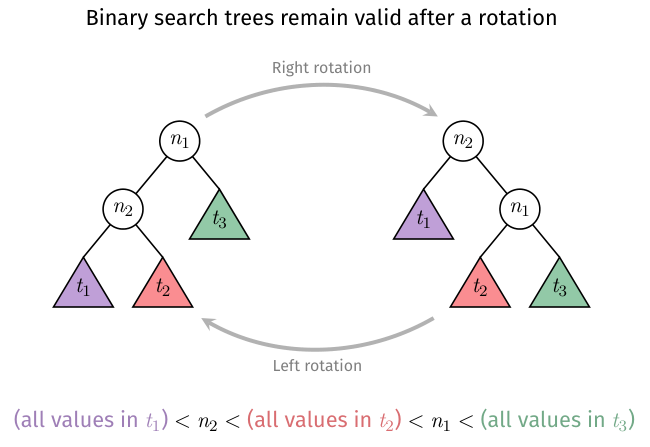
A rotation rearranges two linked nodes and their neighbouring subtrees. It preserves every key and the entire inorder sequence. A right rotation promotes the left child; a left rotation promotes the right child.
In the lecture's general right rotation, the old root is , its left child , and the surrounding subtrees are . Before and after, the ordering is
meaning every key in each named subtree satisfies those inequalities. Notice especially the middle subtree : it was 's right subtree and becomes 's left subtree.
A right rotation in detail#
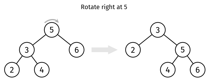
Rotate right at 5 in the pictured tree. The left child 3 becomes the new root; 5 becomes 3's right child. The middle subtree rooted at 4 transfers to 5's left, retaining . Nodes 2 and 6 remain on their outer sides.
/* Uses Node from the BST note. Caller retains the returned root. */
Node *rotateRight(Node *root) {
    if (root == NULL || root->left == NULL) return root;
    Node *newRoot = root->left;
    root->left = newRoot->right;
    newRoot->right = root;
    return newRoot;
}
Node *rotateLeft(Node *root) {
    if (root == NULL || root->right == NULL) return root;
    Node *newRoot = root->right;
    root->right = newRoot->left;
    newRoot->left = root;
    return newRoot;
}
Save the child pointer before altering links. Transfer the middle subtree before connecting the child back to the old root. Otherwise an assignment can overwrite the only route to that subtree or create a cycle. A rotation neither allocates nor frees nodes. Returning a new root is essential: for an internal rotation use, for example, parent->left = rotateRight(parent->left).
This custom lesson uses exactly the lecture's 5,3,2,4,6 example. Each snapshot is a complete valid binary tree. Follow the middle subtree 4 as the root changes:
Vertices: 5, 3, 2, 4, 6. Inorder remains 2,3,4,5,6; no key was copied. Even if the middle subtree had many nodes, only its root pointer moved. Enable JavaScript to inspect each step.
The code and the trace describe the same assignments: newRoot = root->left saves 3, root->left = newRoot->right transfers 4, and newRoot->right = root places 5 beneath 3. The return value reconnects this subtree to its former parent. The trace separates deciding what must happen from the atomic valid-tree snapshot after the links change; it does not pretend an incomplete pointer update is a valid tree.
A rotation performs a fixed number of pointer updates, so costs time and auxiliary space. This remains true for a huge tree because it does not traverse the opaque subtrees. However, one rotation does not necessarily balance the tree: it improves some depths and worsens others. The balancing algorithm must decide where and which way to rotate.
Practice. Rotate left at root 7 whose right child is 23 and whose 23's left subtree is rooted at 16. Where must the 16 subtree go?
Note
- Answer
It becomes 7's right subtree. Every value in it is greater than 7 and less than 23, so it belongs between those two after 23 is promoted. The whole subtree moves by changing one pointer, regardless of how many nodes it contains.
Practice. Why does a plain BST rotation need no copying of key values?
Note
- Answer
Its purpose is to rearrange parent/child links while preserving the same nodes. Values remain in their original allocations. Updating three connections and the returned subtree root changes shape without changing membership or sorted order.
Note
Checkpoint
Right promotes left; left promotes right. Transfer the middle subtree to the old root, retain the new root pointer, and preserve inorder. A constant-time rotation is a tool, not by itself a balance guarantee.
Partition: move a sorted rank to the root#
Here partition is a tree operation, distinct from quicksort's array partition. partition(t,i) moves the item with zero-based rank in inorder to the root using rotations. Its preconditions are a nonempty BST and . Rank counts smaller stored keys; it is not the numeric key itself.
The lecture's rank labels in square brackets distinguish these quantities: root 13 has rank 6, while key 8 has rank 4.
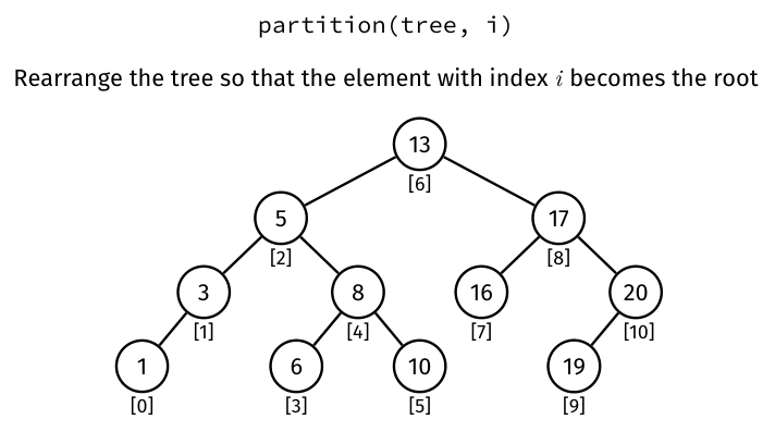
Let be left-subtree size. Then the root's local rank is . If , recursively partition the left child around rank then rotate right. If , partition the right child around rank then rotate left. If , the desired key is already root. The -1 skips the current root after skipping the smaller left-side keys.
partition(t, i):
    L = size(t.left)
    if i < L:
        t.left = partition(t.left, i)
        t = rotateRight(t)
    else if i > L:
        t.right = partition(t.right, i - L - 1)
        t = rotateLeft(t)
    return t
Trace the rank conversion#
The rank-labelled figure above contains eleven keys 1,3,5,6,8,10,13,16,17,19,20. The following trace uses a separate nine-key lecture example, with keys 1,3,5,7,8,10,13,16,17: its middle leaf is 7 rather than 6, and its right subtree omits 19 and 20. In this nine-key tree rooted at 13, partition around rank 4, meaning key 8. Root 13 has six left values, so : descend left to 5, keeping local rank 4. At 5, left size is 2, so go right with rank . At 8, left size is 1, matching the requested local rank, so stop descending.
Unwind: rotate left at 5, promoting 8 above 5. Then rotate right at 13, promoting 8 above 13. The final picture shows that some deeper chains remain: partition chooses a root, not a complete rebalance.
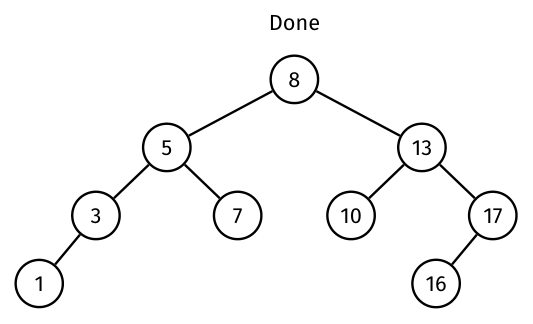
Use the player to follow each comparison and each return-path rotation in that nine-key trace. The active nodes identify the current rank calculation or changed links; the table gives the current local rank, not a count of all keys compared by C.
Vertices: 13, 5, 3, 1, 8, 7, 10, 17, 16. The inorder sequence stays 1,3,5,7,8,10,13,16,17. Partition chooses a root; it does not balance the remaining subtrees. Enable JavaScript to inspect each step.
In C, this player corresponds to partition and sizeRotateLeft/sizeRotateRight below. The selected rank is an argument to the recursive call, and the returned subtree root must be assigned back to t->left or t->right before rotating. There are at most recursive calls and one constant-time rotation per returning level if every subtree size is cached accurately. Without that cache, repeated size traversals can sum to quadratic work on a chain. The few frames here illustrate decisions, not a measured operation count.
Another lecture example has inorder 5,10,14,29,30,32 and asks for rank 3. It selects key 29, not key 3. The return path rotates right at 30, left at 14, then left at 10, bringing 29 to the root. Following the target's old ancestor path gives the required rotation sequence.
Practice. A current subtree has left size 4 and you want local rank 7. Which subtree do you enter and what rank do you request there?
Note
- Answer
Enter the right subtree with rank . Four left keys and the current root precede all right-subtree keys, so they occupy ranks 0 through 4; original rank 7 is the third key on the right.
The cost of asking for size#
The number of rotations is proportional to the target depth, but that alone does not establish the time bound. If size(t->left) traverses the left subtree on every recursive call, a descending chain partitioned around its smallest key computes sizes . Their sum is , even though there are only rotations.
Store each subtree's size in its root instead:
struct sizedNode {
    int item;
    struct sizedNode *left, *right;
    size_t size;
};
Maintain size = 1 + leftSize + rightSize after insertion, deletion and rotations. A null child contributes zero. A right rotation must update the old root first, then the promoted root, since the promoted root's new size depends on its child, the old root. Both updates are .
With valid cached sizes, each partition level takes constant work, giving time and recursive auxiliary space; worst case . Caching is useful only if mutations keep it correct. An old cached size can choose the wrong branch or invalid rank, causing more than a performance problem.
The following executable core uses struct sizedNode above, with assert.h and stddef.h included. Nodes initially need size=1; whenever building or modifying the tree, call sizeUpdate after changing a child. These rotations are separate from the uncached Node functions earlier.
typedef struct sizedNode SNode;
size_t sizeOf(const SNode *t) { return t == NULL ? 0 : t->size; }
void sizeUpdate(SNode *t) {
    t->size = 1 + sizeOf(t->left) + sizeOf(t->right);
}
SNode *sizeRotateRight(SNode *t) {
    assert(t != NULL && t->left != NULL);
    SNode *r = t->left;
    t->left = r->right;
    r->right = t;
    sizeUpdate(t);
    sizeUpdate(r);
    return r;
}
SNode *sizeRotateLeft(SNode *t) {
    assert(t != NULL && t->right != NULL);
    SNode *r = t->right;
    t->right = r->left;
    r->left = t;
    sizeUpdate(t);
    sizeUpdate(r);
    return r;
}
SNode *partition(SNode *t, size_t i) {
    assert(t != NULL && i < sizeOf(t));
    size_t l = sizeOf(t->left);
    if (i < l) {
        t->left = partition(t->left, i);
        t = sizeRotateRight(t);
    } else if (i > l) {
        t->right = partition(t->right, i - l - 1);
        t = sizeRotateLeft(t);
    }
    return t;
}
SNode *sizeRebalance(SNode *t) {
    if (sizeOf(t) < 3) return t;
    t = partition(t, sizeOf(t) / 2);
    t->left = sizeRebalance(t->left);
    t->right = sizeRebalance(t->right);
    sizeUpdate(t);
    return t;
}
size_t is unsigned, so i-l-1 is evaluated only in the branch where i>l; it cannot underflow there. Partition rearranges links without changing the number of nodes in the whole subtree, while rotation updates the two locally changed subtree counts. The rebalance helper implements the global median method developed next.
Note
Checkpoint
Partition uses inorder rank and child sizes to find one node, then lifts it through rotations on the return path. Recomputing subtree sizes can make it quadratic. Maintained size fields reduce the per-level work to constant time.
Global rebalancing#
A global rebalance visits the whole tree and deliberately creates a size-balanced shape. Choose its median key as root using partition at index size/2, then apply the same operation recursively to both child subtrees.
rebalance(t):
    if size(t) < 3: return t
    t = partition(t, size(t) / 2)
    t.left = rebalance(t.left)
    t.right = rebalance(t.right)
    return t
Integer division chooses an upper median for an even number of values. The resulting child sizes differ by at most one. Recursively doing this at every node establishes size balance throughout the tree. Trees with fewer than three nodes already satisfy that condition.
In the lecture example, the seven sorted keys are 2,4,5,8,10,12,15. First bring rank 3, key 8, to root. Its left keys are 2,4,5 and right keys 10,12,15. Recursing chooses 4 and 12 as their roots, producing the final shape pictured on the right.
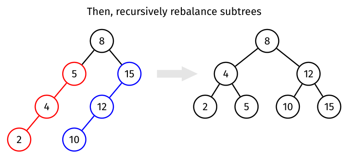
With cached sizes, partitioning a subtree of nodes costs at most . After choosing the median, its children each contain about half the nodes. Thus
At each recursion level the disjoint subtrees total at most nodes; there are median-split levels. This is the lecture's worst-case bound for rotation-based global rebuilding with stored sizes. An initially skewed partition call can still require stack space, despite the final tree having logarithmic height.
A different rebuild variant collects node pointers by inorder into a sorted array and relinks around medians. It can take time but needs auxiliary array space. That is a different algorithm and space trade-off, not the bound of the partition-based method above.
Rebalancing after every insertion is expensive: the rebalance dominates the search. The slide's concrete periodic variant inserts at a leaf, then calls rebalance when the new size is divisible by a chosen positive interval :
periodicInsert(t, v, k):
    t = insertAtLeaf(t, v)
    if a new key was added and size(t) mod k == 0:
        t = rebalance(t)
    return t
The “new key” condition avoids repeatedly rebuilding when a duplicate leaves the size unchanged. This policy gives a balanced shape immediately after each rebuild but no height guarantee between them. The rebuild step may cost with cached sizes, so the worst-case cost of a periodic insertion remains that large. If is fixed, one can amortise rebuilds across batches only after stating a workload and bounding how badly the tree degrades between them; simply dividing rebuild cost by does not prove that all operations are logarithmic.
Rebalancing occasionally reduces rebuilding work but permits a period of worsening shape between rebuilds. Choosing the frequency requires understanding the workload; a single rebuild does not make all future ordinary insertions balanced.
Practice. For six sorted values 1,2,3,4,5,6, which key does partition(t,size/2) choose, and what are the resulting child sizes?
Note
- Answer
Integer 6/2 is rank 3, selecting key 4. There are three smaller keys and two larger keys. The child sizes differ by one, which is allowed. Rank 2, key 3, would also make a valid median-balanced split, but is not the stated variant.
Local methods and what they promise#
Root insertion#
Ordinary insertion puts a new node at a leaf. Root insertion follows the same comparison path but rotates the inserted node upward at each return, ending with it at the root:
Node *insertAtRoot(Node *t, int v) {
    if (t == NULL) return newNode(v);
    if (v < t->item) {
        t->left = insertAtRoot(t->left, v);
        t = rotateRight(t);
    } else if (v > t->item) {
        t->right = insertAtRoot(t->right, v);
        t = rotateLeft(t);
    }
    return t;
}
This excerpt uses the ordinary BST Node and uncached rotations. If using cached metadata, also update it. The lecture's larger example inserts 24 into the BST with keys 5,10,14,29,30,32. The next player shows the descent and all four return-path rotations. Follow the newly allocated 24, then inspect the final tree's remaining depth; the operation promotes recency without enforcing an AVL invariant.
Vertices: 10, 5, 14, 30, 29, 32. Recent key 24 is now at depth 0, but the right branch still has depth 2. Root insertion does not guarantee AVL balance. Enable JavaScript to inspect each step.
The C function performs one comparison at each visited ancestor and at most one rotation on each return, giving time and recursive stack space. Its four trace rotations are for this particular input, not a constant bound for arbitrary . The final inorder check establishes the BST ordering; it does not prove balance.
For a new key 4 inserted into the tree containing root 5 and left 2, the path goes 5→2→null on the right. Create 4, rotate left at 2, then right at 5. Root becomes 4 with children 2 and 5.
For an existing value, no new node is created. The recursive code can still rotate that existing value upward through its ancestors; membership stays the same. This is a structural effect that a client must not confuse with inserting a duplicate occurrence.
There are comparisons and at most one constant-time rotation per ancestor, giving time and stack space. It is attractive when newly added items are likely to be searched soon because those items move near the root.
But ascending insertions still make a chain: insert 1, then 2 becomes root with left 1, then 3 becomes root above 2, and so on. Root insertion changes which end is shallow; it does not guarantee height balance.
Practice. After root-inserting 1,2,3,4, what is the height? Which search becomes cheap and which remains long?
Note
- Answer
Root 4 has left child 3, whose left child is 2, whose left child is 1. Height is 3. Searching for 4 is constant time; searching for 1 follows every node. Root insertion favours recent arrivals but has not reduced worst-case height.
Randomised root-or-leaf insertion#
The lecture introduces a heuristic: randomly choose normal insertion or root insertion. For a probability , choose root insertion when a pseudorandom result modulo is smaller than ; otherwise choose normal leaf insertion. Its 30% example uses .
The aim is to make shape less tightly determined by an externally supplied insertion order. A pseudorandom generator is an algorithm that produces a repeatable sequence from a seed; apparent randomness is not an invariant forcing balance. Particular outcomes can still produce a chain, so the method has no worst-case logarithmic guarantee.
Do not infer an exact expected theorem merely from the fixed 30% mixture. A standard random-BST distribution algorithm uses size-dependent root probabilities within recursive insertion; that is a different variant. For the lecture heuristic, the justified statements are constant-factor path overhead, possible shape improvement, and retained worst-case operations.
| Method | What is controlled | Main cost/limitation |
|---|---|---|
| Ordinary insertion | BST ordering | Can produce a chain |
| Global median rebalance | Size balance after the rebuild | lecture rebuild with cached sizes |
| Root insertion | New key moves to root | ; still permits chains |
| Random root/leaf choice | Reduces direct dependence on order heuristically | No worst-case balance guarantee |
| [[11. AVL Trees | AVL insertion/deletion]] | Height balance after every operation |
Practice. Why does “one rotation costs constant time” not imply “maintaining a tree costs constant time per operation”?
Note
- Answer
We first need to locate the relevant node and may rotate along a path with many ancestors. Path length can be linear in an unbalanced tree. The operation count must include search, metadata work and all rotations, not just one local step.
More exam-style practice#
Work each prompt before opening its answer. State the invariant or cost assumption that makes your reasoning valid.
Question 1. Rotate right at root 30 whose left child is 20 and whose left child has right subtree rooted at 25. State the three changed links.
Note
- Answer
Let x=20 and B=25. Set 30->left=B, then 20->right=30, and return 20 as the new subtree root. The inorder order remains 20,25,30, with any subtrees under those nodes remaining in their intervals.
Question 2. A BST of 15 keys is a chain. If rebuilding it into a near-perfect BST costs Θ(n), what heights before and after do you expect?
Note
- Answer
Before rebuilding, the longest root-to-leaf path contains 15 nodes, so edge-height is 14 (or node-height 15). A near-perfect 15-node BST has four levels, edge-height 3. Search changes from Θ(n) worst case to Θ(log n) after the rebuild.
Question 3. Why does a routine that recomputes subtree sizes recursively at every step of rank-based partitioning risk more than logarithmic work?
Note
- Answer
Even if the path has logarithmic depth in a balanced tree, recomputing a size can scan much of its subtree repeatedly. Store sizes as metadata and update them after structural changes, or account for the repeated scans explicitly. Counting only recursive path length hides this cost.
Note
Checkpoint
Global median partitioning buys a deliberate balanced shape by processing the whole tree. Root insertion and a random mixture make local changes without a balance guarantee. AVL trees add an enforceable invariant so path lengths remain logarithmic after every update.