16. Minimum Spanning Trees
Connecting Every Vertex as Cheaply as Possible#
A spanning tree of an undirected connected graph keeps all vertices and enough edges to connect them without cycles. With vertices it has exactly edges. A minimum spanning tree (MST) is a spanning tree with the smallest possible total edge weight.
An MST models the cost of building a connected network: cables linking computers, power lines linking locations, or roads connecting towns. We pay once for each selected edge. This objective differs from finding short routes from one source to every destination.
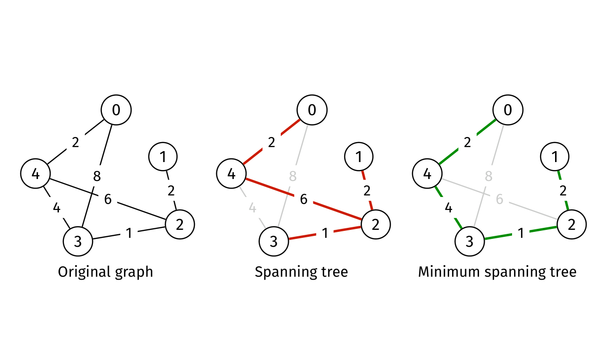
The middle tree connects all five vertices with total cost . The right tree connects the same vertices with cost . Both have four edges and are acyclic; the right one improves the sum, not the edge count.
MST algorithms assume undirected input. Negative and zero weights are allowed: we still select just edges, so there is no repeated negative-cycle traversal issue. If a graph is disconnected, no single spanning tree exists; the corresponding output is a minimum spanning forest, one MST per component. State whether a function reports disconnectedness or returns that forest.
If several edges have equal weights, several different MSTs may have the same minimum cost. All distinct weights guarantee uniqueness; the converse is false—a graph can still have a unique MST when some weights tie.
Practice. Is an MST necessarily a shortest-path tree from vertex 0?
Note
- Answer
No. For a triangle with of weight 2, of weight 2, and of weight 3, an MST uses the first two edges, cost 4. Its route from 0 to 2 costs 4, but the original direct edge has cost 3. A shortest-path tree from 0 chooses the direct edge and costs 5 in total. The objectives differ.
Greedy Choices and the Cut Property#
A greedy algorithm repeatedly makes the best immediate choice according to a rule. That alone does not prove global optimality: choosing a locally cheap edge could be wrong unless the rule makes the choice safe.
A cut separates the vertices into a nonempty set and its complement. An edge crosses the cut when exactly one endpoint lies in . If the graph is connected, at least one edge crosses any such cut. The cut property says a minimum-weight crossing edge is safe to include in some MST, provided the cut does not split any already selected edge.
Why? Take an MST containing the earlier selected edges. If it already contains the chosen edge , nothing needs changing. Otherwise add to , which creates one cycle. That cycle has another edge crossing the cut: to return to its starting side, it must cross back. Because is a cheapest crossing edge, . Remove . The resulting graph is again a spanning tree, still contains the earlier choices, and costs no more. Thus we can preserve an optimal solution while accepting .
This is an exchange argument: modify an alternative optimal solution until it agrees with the greedy choice, without increasing cost. It proves safe choices exist; it does not claim every cheap edge can always be selected.
Note
Checkpoint
An MST minimises the total cost of an acyclic connected network. The cut property justifies local greedy choices by exchanging an edge in an optimal tree. Equal weights can give different valid minimum trees.
Kruskal's Algorithm#
Grow a Forest in Weight Order#
Kruskal begins with every vertex isolated. Sort edges into nondecreasing weight order. For each edge , add it if its endpoints are currently in different components of the selected forest. If they are already connected, adding it would close a cycle, so reject it. For a connected graph, stop after accepting edges.
The lecture gives two equivalent checks:
- Temporarily insert the edge, check for a cycle, and remove it if necessary.
- Before insertion, search the current forest for a path between its endpoints. Insert only if no path exists.
Checking the original graph would reject almost everything in a connected graph. We test the selected forest, because it describes what has already been purchased.
A Worked Lecture Trace#
Use the five-vertex graph with edges , , , , , , , .
| Edge considered | Selected-forest decision | Components afterwards | Total cost |
|---|---|---|---|
| , weight 1 | Accept: separate singleton components | 1 | |
| , weight 2 | Accept: 3 and 4 are separate | 3 | |
| , weight 3 | Accept: connects two groups | 6 | |
| , weight 4 | Reject: route already exists | Same | 6 |
| , weight 5 | Reject: route already exists | Same | 6 |
| , weight 6 | Accept: joins the final singleton | 12 |
Four accepted edges equal , so stop. The remaining weights 7 and 8 need not be tested.
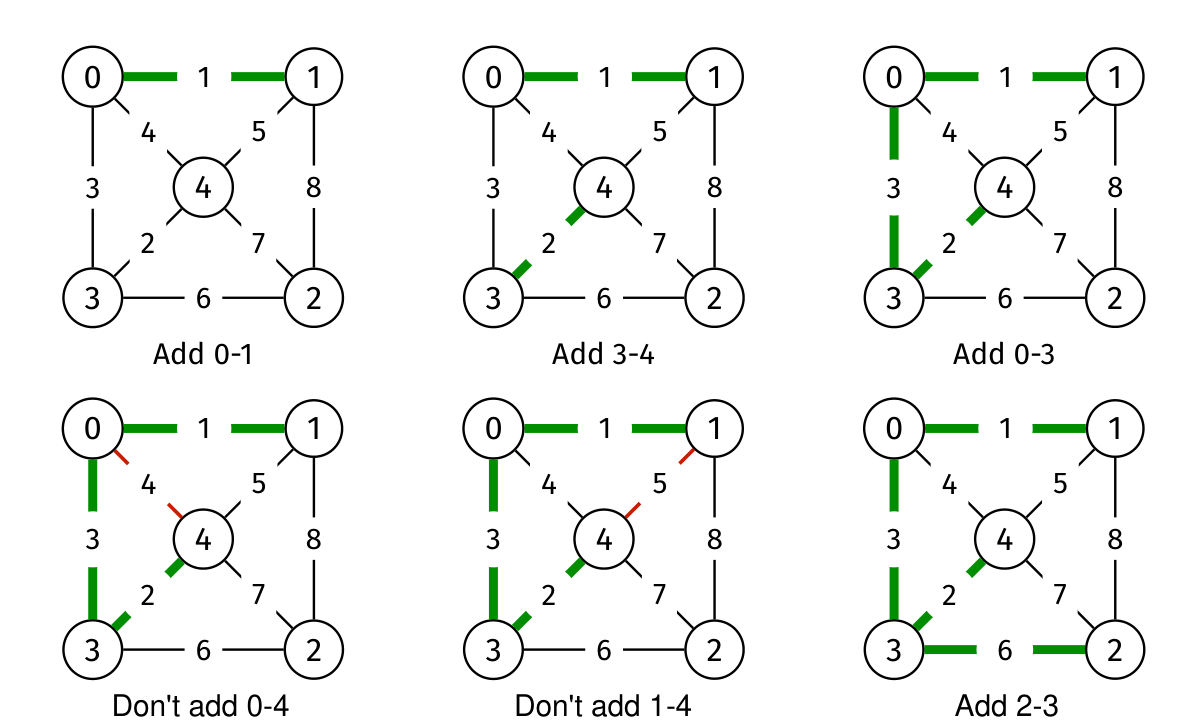
Green edges form the current forest. A red candidate is rejected when its endpoints are already linked by green edges. At no stage must the selected forest be connected; connecting the separate groups is the algorithm's purpose.
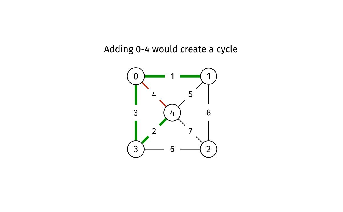
In particular, edge has weight 4 and is fairly cheap, but already joins its endpoints. Adding it would create cycle and fail the tree constraint.
The custom lesson below follows the lecture's path-checking version. It makes the selected-forest route explicit and stops at four accepted edges. The built-in Kruskal uses union-find and scans the full sorted edge sequence; that is a useful alternative, but would teach different state and stopping behaviour here.
Vertices: 0, 1, 2, 3, 4. Stop: the connected forest has V-1=4 edges, so it is an MST. The remaining weights 7 and 8 need no checks. Enable JavaScript to inspect each step.
Practice. Why is rejected even though its weight 4 is lower than the accepted weight 6 of ?
Note
- Answer
The rejection is about cycles, not an absolute weight cutoff. Edge duplicates a connection within an already connected group. Edge is needed to join vertex 2 to that group. Removing its weight-6 connection would leave 2 isolated; replacing it with would not repair that.
Correctness and Costs#
Maintain the invariant that the selected graph is a forest and can be extended to an MST. A rejected edge preserves that forest unchanged. For an accepted edge, take the cut whose one side is a selected component containing one endpoint. All earlier cheaper edges crossing that cut would already have joined the groups; none remains available that is strictly cheaper. The candidate is therefore a cheapest available crossing edge for a cut respecting earlier selections. The exchange argument preserves an optimal extension. After accepted edges in a connected graph, that forest is a spanning tree and hence an MST.
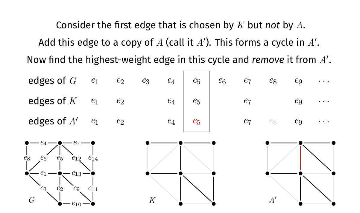
Read as Kruskal's choices, as an alternative tree, and as the modified alternative. The new edge creates a cycle; removing a suitable no-cheaper edge restores a tree. The ordering argument ensures the exchange can retain earlier agreed choices. Repeating makes an optimal alternative agree with all of .
Sorting edges using an efficient comparison sort costs . There are at most candidate checks. The selected graph is always a forest, so it has at most edges. A DFS on its adjacency lists costs , not using the original graph's edge count. The lecture variant therefore costs
for simple graphs, since makes and . A matrix-based forest search can instead cost per candidate, giving a looser bound. Representation still matters even though the forest is sparse.
Union-find, also called disjoint-set union, stores component representatives instead of rerunning DFS. find(v) returns its component representative; union(u,v) merges two groups. With path compression and union by rank, the total operation cost is near-linear, expressed as amortised, where is the extremely slowly growing inverse Ackermann function. This is not literally constant worst-case time per operation. Together with sorting, the usual connected-graph Kruskal bound is . Initialising singleton sets must still be counted for graphs with many isolated vertices.
Prim's Algorithm#
Grow One Connected Tree#
Prim starts from any vertex. Keep a set used containing the vertices already in the tree. Repeatedly choose the cheapest edge with one endpoint used and the other unused. Add that edge and the unused endpoint. Stop after all vertices are included, or after edges.
The candidate edges cross the cut (used, unused). An edge with both endpoints used would create a cycle; one with neither endpoint used would start a separate tree instead of growing this one. Prim's choices keep the current tree connected.
On the earlier graph, starting from 0:
| Used vertices before choice | Eligible edges and their weights | Choice |
|---|---|---|
| , , | ||
| , , , | ||
| , , , , | ||
| , , |
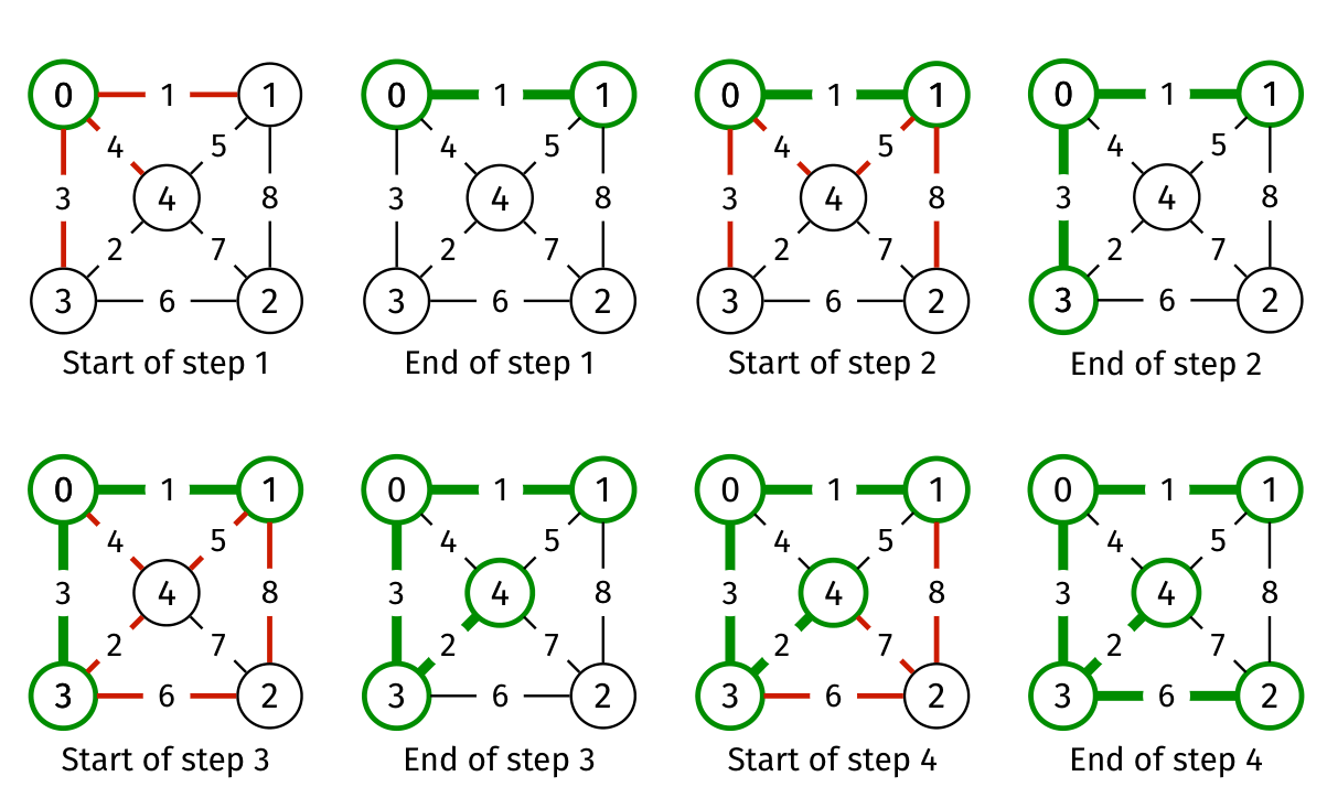
The weight-2 edge is chosen after the weight-3 edge because it did not touch the current tree earlier. Thus Prim's accepted weights need not increase. Kruskal's globally sorted order and Prim's changing boundary can produce the same final MST in different orders.
The built-in below rescans the edge set for the minimum boundary edge, matching the lecture's basic variant. For this connected graph it grows from 0 throughout. It also supports disconnected inputs by restarting at another vertex and returning a forest.
Vertices: 0, 1, 2, 3, 4. Minimum spanning forest complete: 4 edges connect 1 component(s) with total weight 12. Enable JavaScript to inspect each step.
Its invariant is that the selected tree is connected, covers exactly the used vertices, and has an optimal extension. The chosen edge is the cheapest across the used/unused cut, so the cut property preserves that extension. It adds one new vertex and cannot create a cycle. After all vertices are used, the tree is minimum.
If no boundary edge exists while unused vertices remain, the graph is disconnected. The lecture pseudocode assumes connected input, so it would otherwise have no valid next edge. A robust implementation must stop and report this, or start another component for a forest.
Practice. Why can Prim not choose of weight 2 in its first step from 0?
Note
- Answer
Neither endpoint is used yet. It does not cross the current cut versus the rest, so it cannot extend the current tree. After is selected, vertex 3 is used and becomes eligible.
C Implementations of the Lecture Variants#
The following bounded teaching implementation stores a selected forest using adjacency lists, with at most list entries. Each undirected accepted edge contributes two entries. The integer next field is a list index; -1 means end of list. This gives the same neighbour-following operation as pointer lists, while avoiding allocation for each small node.
It accepts 1–32 vertices and a supplied array of valid, loop-free undirected edges. The input is not modified. Negative weights work, and long long safely stores at most 31 int weights. chosen records the result edges, while head/links support selected-forest path checks.
#include <assert.h>
#include <stdbool.h>
#include <stdlib.h>

#define MST_MAXV 32
typedef struct { int u, v, weight; } Edge;
typedef struct { int to, next; } Link;
typedef struct {
    int n, count, usedLinks;
    int head[MST_MAXV];
    Link links[2 * (MST_MAXV - 1)];
    Edge chosen[MST_MAXV - 1];
    long long cost;
} Forest;

static Forest emptyForest(int n) {
    assert(n > 0 && n <= MST_MAXV);
    Forest f = {.n = n};
    for (int v = 0; v < n; v++) f.head[v] = -1;
    return f;
}
static void addForestEdge(Forest *f, Edge e) {
    assert(f->count < f->n - 1);
    f->chosen[f->count++] = e;
    f->cost += e.weight;
    f->links[f->usedLinks] = (Link){e.v, f->head[e.u]};
    f->head[e.u] = f->usedLinks++;
    f->links[f->usedLinks] = (Link){e.u, f->head[e.v]};
    f->head[e.v] = f->usedLinks++;
}
static bool forestPath(const Forest *f, int v, int target, bool seen[]) {
    if (v == target) return true;
    seen[v] = true;
    for (int i = f->head[v]; i != -1; i = f->links[i].next) {
        int w = f->links[i].to;
        if (!seen[w] && forestPath(f, w, target, seen)) return true;
    }
    return false;
}
static void checkInput(int n, const Edge edges[], int m) {
    assert(n > 0 && n <= MST_MAXV && m >= 0);
    assert(m == 0 || edges != NULL);
    for (int i = 0; i < m; i++) {
        assert(edges[i].u >= 0 && edges[i].u < n);
        assert(edges[i].v >= 0 && edges[i].v < n);
        assert(edges[i].u != edges[i].v);
    }
}
static int edgeCompare(const void *pa, const void *pb) {
    const Edge *a = pa, *b = pb;
    if (a->weight != b->weight)
        return (a->weight > b->weight) - (a->weight < b->weight);
    if (a->u != b->u) return (a->u > b->u) - (a->u < b->u);
    return (a->v > b->v) - (a->v < b->v);
}

Forest kruskal(int n, const Edge edges[], int m) {
    checkInput(n, edges, m);
    Forest f = emptyForest(n);
    if (m == 0) return f;
    Edge *sorted = malloc((size_t)m * sizeof *sorted);
    if (sorted == NULL) exit(EXIT_FAILURE);
    for (int i = 0; i < m; i++) sorted[i] = edges[i];
    qsort(sorted, (size_t)m, sizeof *sorted, edgeCompare);
    for (int i = 0; i < m && f.count < n - 1; i++) {
        bool seen[MST_MAXV] = {false};
        Edge e = sorted[i];
        if (!forestPath(&f, e.u, e.v, seen)) addForestEdge(&f, e);
    }
    free(sorted);
    return f; // a minimum forest if disconnected
}

Forest prim(int n, const Edge edges[], int m, int start) {
    checkInput(n, edges, m);
    assert(start >= 0 && start < n);
    Forest f = emptyForest(n);
    bool used[MST_MAXV] = {false};
    used[start] = true;
    while (f.count < n - 1) {
        int best = -1;
        for (int i = 0; i < m; i++) {
            Edge e = edges[i];
            if (used[e.u] != used[e.v] &&
                (best == -1 || e.weight < edges[best].weight)) best = i;
        }
        if (best == -1) break; // disconnected: return source-component tree
        Edge e = edges[best];
        addForestEdge(&f, e);
        used[e.u] = used[e.v] = true;
    }
    return f;
}
Kruskal returns a minimum forest on disconnected input. This C Prim returns only the source-component tree and its unused isolated vertex slots; check f.count == n-1 before treating it as a full MST. The player instead restarts to form a complete minimum forest. These return contracts are explicit so an incomplete result cannot be mistaken for a spanning tree.
The comparator uses relational comparisons rather than subtracting weights, which could overflow when comparing large positive and negative integers. qsort provides a convenient library sort; the ISO C contract does not promise a particular time bound. The analysis assumes an efficient comparison-sort implementation. To enforce that bound independently of the C library, use a worst-case mergesort or heapsort from the sorting notes.
For this bounded storage, MST_MAXV is a capacity, not the actual input size. A scalable version reserves list space proportional to and edge-copy space proportional to . Kruskal then uses extra storage including the copied edges and result; each forest search requires temporary marks and call depth. Reusing the mark array does not reuse its visited state: each candidate needs a fresh endpoint search.
Prim's Costs and Choosing a Variant#
The C Prim scans all edges for every accepted vertex. There are at most acceptances and possibly one final unsuccessful scan, so the bound is , normally written for nontrivial connected graphs. It stores selected-tree state and marks, excluding the input edge array. Scanning all edges is simple, but expensive on a dense graph.
Another implementation maintains best[v], the cheapest edge joining each unused vertex to the used set, and parent[v]. With an adjacency matrix, choosing the next minimum best and updating one row each costs per added vertex, yielding overall. Notice the difference from Dijkstra: Prim's key is one joining edge, while Dijkstra's key is a whole route from the source.
With adjacency lists and an indexed binary heap, Prim has time: removals and up to key decreases. A Fibonacci heap makes decreases amortised and minimum removals amortised, giving . The lecture's advanced comparison refers to this Fibonacci-heap implementation, not the simple edge-rescanning code or the built-in player. The more complex representation can be beneficial on dense graphs, but theoretical bounds alone do not predict every practical implementation's speed.
| Variant being compared | Time with its stated assumptions |
|---|---|
| Kruskal, selected-forest list DFS | |
| Kruskal, efficient sort and union-find | |
| Prim, rescan edge array | |
| Prim, matrix plus minimum-key scan | |
| Prim, lists plus binary heap | |
| Prim, lists plus Fibonacci heap | amortised |
The slide's versus comparison uses the advanced Kruskal and Prim variants. In a sparse connected graph, sorting an edge list is attractive. For a dense graph already stored as a matrix, Prim can be a straightforward choice without building a complicated heap. Always compare like-for-like representations and operations.
Practice. In the triangle , , , what key does Prim give vertex 2 after adding vertex 1? What distance does Dijkstra give it?
Note
- Answer
Prim changes vertex 2's joining-edge key from 3 to 2, because edge is cheaper than . Dijkstra compares the source-route cost with the direct cost 3 and keeps 3. Prim pays for the cheapest next network link; Dijkstra minimises a complete source route.
Other MST Algorithms Named in the Slides#
Borůvka's algorithm begins with singleton components. In a round, each component chooses a cheapest outgoing edge, and those safe connections merge groups. An implementation handles repeated chosen edges and ties so adding them preserves a forest. Components with outgoing edges at least halve in number each round, producing rounds; scanning all edges per round gives for connected graphs. For disconnected graphs it stops with a minimum spanning forest.
The lecture also names the Karger–Klein–Tarjan randomized MST algorithm, based on Borůvka-style reductions and random edge sampling, with expected linear time. “Expected” means averaging over the algorithm's random choices, not assuming that input graphs arrive in a particular favourable distribution. Its full construction is outside these decks; do not infer that ordinary Kruskal or Prim has that bound.
More exam-style practice#
Work each prompt before opening its answer. State the invariant or cost assumption that makes your reasoning valid.
Question 1. For edges AB=1, BC=2, AC=3, CD=4, BD=5, run Kruskal’s selection in weight order.
Note
- Answer
Choose AB and BC, skip AC because A, B and C are already connected and it would form a cycle, then choose CD. The MST edges are AB,BC,CD with total weight 7.
Question 2. Prim’s current tree contains A and B. Crossing edges are A–C=8, B–C=3, B–D=5; which edge is safe to choose next, and why?
Note
- Answer
Choose B–C=3, the minimum edge crossing from the current tree to outside vertices. The cut property guarantees a minimum crossing edge belongs to some MST; choosing an arbitrary globally small edge that does not cross this cut is not Prim’s step.
Question 3. A triangle has AB=2, AC=2 and BC=1. Find an MST and a shortest-path tree rooted at A. Compare their total weights and A-to-C distances.
Note
- Answer
An MST takes BC and either AB or AC, total weight 3. If it takes AB, its A-to-C path costs 2+1=3. The shortest-path tree rooted at A takes AB and AC, total weight 4, but A reaches both B and C at distance 2. The two objectives are different.
Question 4. Explain the difference between O(E log E) Kruskal sorting work and the near-constant union-find checks.
Note
- Answer
Sorting all E edges dominates the standard implementation. Cycle checks and unions operate on disjoint-set roots with amortised O(α(V)) each under path compression and rank/size heuristics, for O(E α(V)) additional work. The bounds describe distinct phases.
Note
Checkpoint
Kruskal processes globally sorted edges and grows a forest. Prim grows one tree by the cheapest current boundary edge. Both rely on safe cut choices, not shortest-path reasoning. Their time bounds change with cycle checks, graph storage, and priority-update implementation.