15. Directed Graph Algorithms and Shortest Paths
Direction Changes Reachability#
An edge allows travel from to . It does not imply . BFS and DFS still work: iterate only over the current vertex's outgoing neighbours. Their adjacency-list bounds remain , where counts vertices and counts directed edges. Each edge is now stored and scanned once, rather than twice as in an undirected graph.
Directed reachability is not symmetric. In , source 0 reaches every vertex, but source 2 reaches only itself. One search reaching every vertex does not establish strong connectivity, which requires a route from every vertex to every other vertex.
A strongly connected component (SCC) is a maximally strongly connected group. Any two vertices within one SCC can reach each other in both directions. A one-vertex SCC is possible without a loop, using the zero-edge path from the vertex to itself.
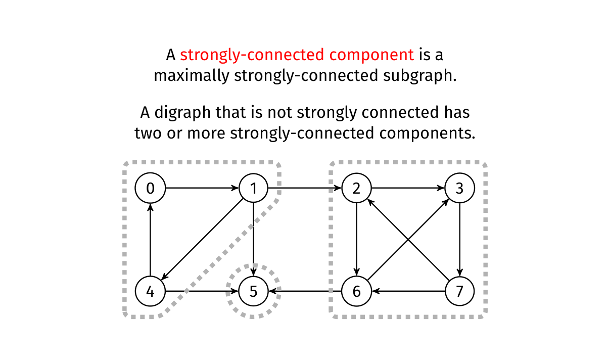
The left SCC is , the right SCC is , and vertex 5 forms an SCC on its own. Arrows between the groups do not merge them unless travel becomes possible in both directions. For example, an outgoing route from the left group into the right group is insufficient if there is no route back.
The undirected component-label test in 14. Graph Problems therefore cannot simply be reused. If the labels mean SCC membership, unequal labels do not imply no one-way route: different SCCs can still be joined by directed paths. The slides name Kosaraju's and Tarjan's algorithms as further SCC algorithms; their detailed implementations are outside these decks. Once a reachability matrix is available, mutual reachability gives a simple conceptual SCC test: or both tc[s][t] and tc[t][s].
Practice. In , , , which SCCs exist? Is 2 reachable from 0?
Note
- Answer
The SCCs are and . Vertex 2 is reachable from 0 along , but it cannot reach either 0 or 1. SCC membership describes mutual reachability, not every possible one-way route.
Web Crawling as Directed BFS#
A webpage is a vertex; each hyperlink is an outgoing edge. A crawler usually does not know the full vertex set beforehand, so an integer-indexed visited array is unsuitable. Maintain a visited set of URLs instead, using a search structure such as a hash table from 17. Hash Tables. Add a URL to that set when it is enqueued, preventing several pages from scheduling it repeatedly.
The lecture crawler dequeues a URL, visits the page, enqueues each unseen hyperlink, and stops when the queue empties or a page budget is reached. BFS explores pages close to the starting page first; DFS may spend the whole budget on a long branch. In the Wikipedia-click game, BFS finds a fewest-click route because links are unweighted. Network retrieval time and URL processing are additional costs; describes the graph operations under constant-time neighbour and membership assumptions, not the total latency of downloading the web.
Transitive Closure: Precompute Routes#
An adjacency matrix answers “is there an edge from to ?”. A transitive closure matrix, tc, answers “is there a route from to ?”. If reachability is queried often and the graph changes rarely, spending time to construct this matrix can save repeated traversals.
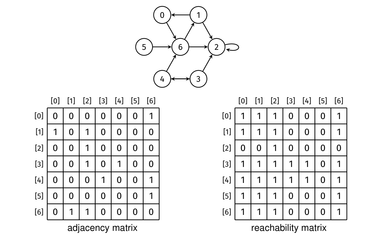
Read rows as sources and columns as destinations. The left table records immediate edges. The right table records routes through any number of intermediate vertices. A true entry in the right table does not mean a new physical edge was inserted into the original graph.
There are two conventions for self-reachability:
- Positive-length transitive closure: start from adjacency alone;
tc[v][v]is true only when a nonempty directed route returns to . - Reflexive transitive closure: also initialise every diagonal entry to true, allowing the empty path.
The lecture's Warshall pseudocode copies the adjacency matrix without adding the identity matrix. Its worked example leaves some diagonal entries false. We follow that positive-length convention below. Ordinary DFS/BFS path checking, meanwhile, treats a source as reachable from itself using the empty path. These operations answer slightly different questions; neither convention should be silently swapped for the other.
Warshall's Algorithm#
The transitivity rule is: if reaches and reaches , then reaches . Warshall makes this systematic by allowing one more intermediate vertex at each stage.
At the start, only direct edges are known. After stage , tc[s][t] means a route exists whose intermediate vertices belong to . An intermediate vertex is between the endpoints: on , and are intermediate, while and are endpoints.
For every pair , preserve a known route or join routes through the newly allowed vertex :
The outer loop must be the intermediate-vertex loop. Simply permuting the three loops can invalidate the staged meaning and miss paths.
The Lecture's Four-Vertex Trace#
The starting edges are , , , . Each row below is ordered by destination 0,1,2,3.
| Stage | Row 0 | Row 1 | Row 2 | Row 3 | Newly established routes |
|---|---|---|---|---|---|
| Adjacency | 0010 |
1001 |
0000 |
0100 |
Direct edges |
0010 |
1011 |
0000 |
0100 |
via 0 | |
0010 |
1011 |
0000 |
1111 |
, , via 1 | |
0010 |
1011 |
0000 |
1111 |
None: 2 has no outgoing route | |
0010 |
1111 |
0000 |
1111 |
via 3 |
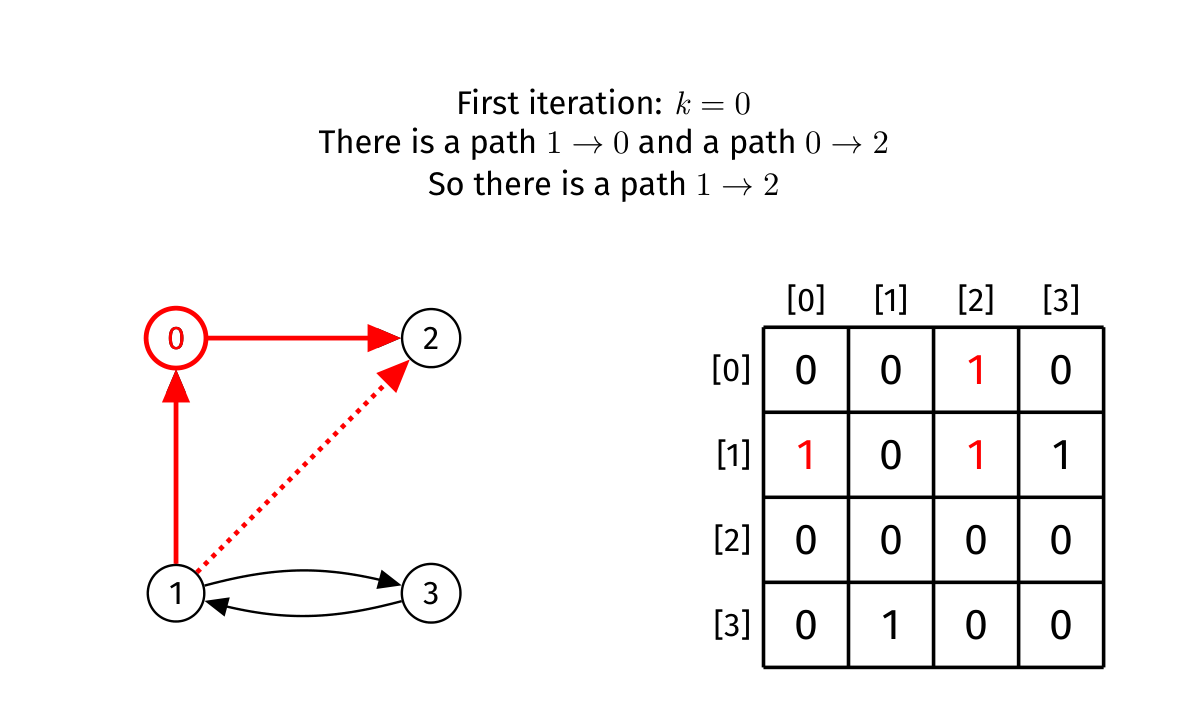
At , tc[1][0] and tc[0][2] are true, so set tc[1][2]. This is the route .
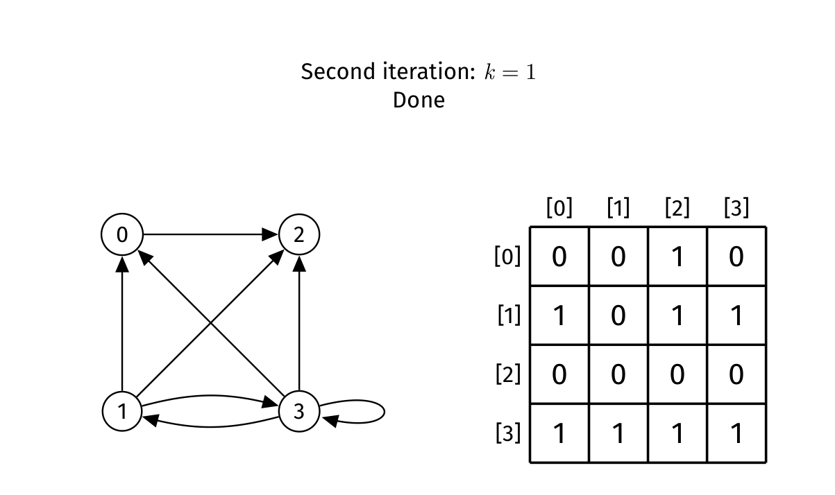
At , vertex 3 reaches 1, whose row now says it reaches 0, 2 and 3. Therefore row 3 gains those three entries. In particular makes tc[3][3] true. No identity matrix was inserted: the diagonal entry comes from an actual cycle.
The custom player retains the original graph and shows the closure in its table. Step through the allowed-intermediate stages; the table rows use the same destination order as the static trace.
Vertices: 0, 1, 2, 3. The final table answers positive-length reachability queries in constant time. Enable JavaScript to inspect each step.
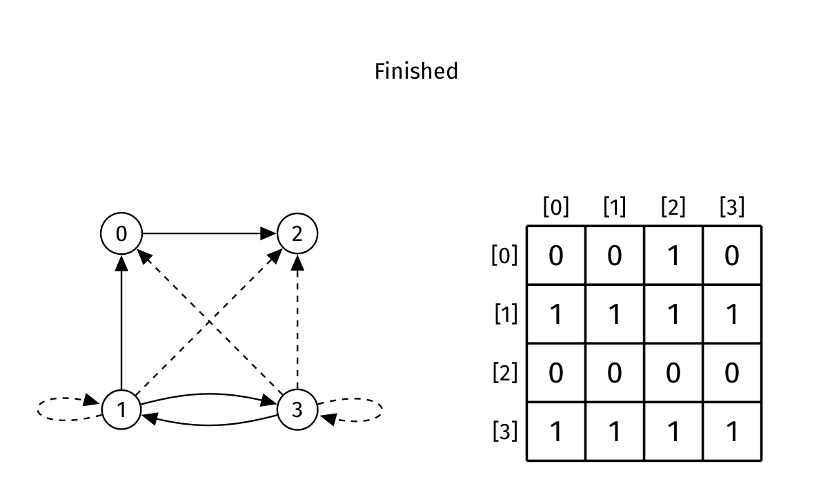
Practice. Why does tc[0][0] remain false, despite vertex 0 being reachable from itself in ordinary path checking?
Note
- Answer
This closure starts with direct edges and records positive-length routes. Vertex 0 leads to 2, which has no outgoing edge; no nonempty route returns to 0. To include the empty path, initialise tc[v][v]=true for every vertex before the stages. That would intentionally compute reflexive closure instead.
C Implementation and Correctness#
The following independent examples use bounded matrices of up to 32 vertices. They keep source data separate from closure data.
#include <assert.h>
#include <stdbool.h>
#include <limits.h>

#define MAXV 32
typedef struct {
    int n;
    bool edge[MAXV][MAXV];
} Digraph;

void warshall(const Digraph *g, bool tc[MAXV][MAXV]) {
    assert(g->n > 0 && g->n <= MAXV);
    for (int s = 0; s < g->n; s++)
        for (int t = 0; t < g->n; t++)
            tc[s][t] = g->edge[s][t];
    for (int k = 0; k < g->n; k++)
        for (int s = 0; s < g->n; s++)
            for (int t = 0; t < g->n; t++)
                if (tc[s][k] && tc[k][t]) tc[s][t] = true;
}
Why does it work? Assume the table correctly represents routes using only intermediates smaller than . A route allowed at the next stage either avoids , in which case it was already represented, or passes through . Split that route at : its two halves use only earlier intermediates and are represented by tc[s][k] and tc[k][t]. Joining them establishes exactly the new possibility. For existence, repeated sections can be removed; positive-length self-routes are represented by cycles. Induction over the stages proves the final matrix.
In-place updates are safe for this Boolean recurrence. During stage , its row and column do not acquire any previously false entry through itself: the update for tc[s][k] is tc[s][k] || (tc[s][k] && tc[k][k]), which equals the existing value. The same applies to tc[k][t]. Thus later checks in the stage do not accidentally use a new, unsupported row or column state.
There are choices of , and endpoint pairs for each, giving checks. Copying the input adds . The result matrix requires storage; additional workspace is if the input matrix itself may be overwritten. Overwriting adjacency destroys the distinction between an edge and a route, so use a separate table when later operations still need the original edges.
Running BFS/DFS independently from each source instead costs with lists, plus storing or initialising the answers. This can be preferable for sparse graphs. Once either result is built, one reachability query is . An edge insertion or deletion can change many answers, so cached closure needs maintenance or rebuilding.
Note
Checkpoint
Warshall expands the permitted intermediate set one vertex at a time. Keep outermost and distinguish adjacency from reachability. The lecture's closure includes positive-length routes; choose diagonal initialisation deliberately. Preprocessing costs cubic time but makes subsequent queries constant-time.
Topological Order and Directed Cycles#
The digraph lecture names topological sorting as a further algorithm. This section provides a concrete extension so task-dependency graphs are usable rather than just named.
A topological order of a digraph lists every vertex so that, for each edge , appears before . If edges mean “must finish before”, this is a valid task order. Such an order exists exactly for a directed acyclic graph (DAG), a directed graph with no directed cycle.
A cycle would require before , before , and before , which no linear order can satisfy. Undirected parent-skipping cycle detection does not solve this problem: an edge to an already visited directed vertex might merely point to an earlier completed branch.
Kahn's Indegree Algorithm#
Count incoming edges for each vertex. Enqueue every vertex with indegree zero: it has no remaining prerequisite. Remove one, append it to the answer, then decrement the indegree of each outgoing neighbour. When a neighbour's indegree reaches zero, enqueue it. Stop when the queue empties.
Example: , , , , . Initial indegrees are A:0, B:0, C:2, D:1, E:2. With ready queue [A,B], remove A: C falls to 1. Remove B: C and D reach 0, yielding [C,D]. Remove C: E falls to 1. Remove D: E reaches 0. Then remove E. One result is A,B,C,D,E; other valid orders exist.
Vertices: A, B, C, D, E. Topological order complete; every edge points from an earlier vertex to a later one. Enable JavaScript to inspect each step.
Follow how readiness depends on all incoming prerequisites, rather than merely the last edge inspected. The built-in implements this FIFO indegree variant. It rejects cyclic inputs because a complete topological order would be impossible.
// Uses Digraph above. Writes all vertices if acyclic; otherwise
// writes only the removable prefix and returns false.
bool topological(const Digraph *g, int order[]) {
    assert(g->n > 0 && g->n <= MAXV);
    int indegree[MAXV] = {0}, queue[MAXV];
    int front = 0, rear = 0, count = 0;
    for (int v = 0; v < g->n; v++)
        for (int w = 0; w < g->n; w++)
            indegree[w] += g->edge[v][w] ? 1 : 0;
    for (int v = 0; v < g->n; v++)
        if (indegree[v] == 0) queue[rear++] = v;
    while (front < rear) {
        int v = queue[front++];
        order[count++] = v;
        for (int w = 0; w < g->n; w++)
            if (g->edge[v][w] && --indegree[w] == 0)
                queue[rear++] = w;
    }
    return count == g->n;
}
The invariant is that every listed vertex has had all predecessors listed already; the ready queue contains vertices with no incoming edge from the unlisted subgraph. If vertices remain but no zero-indegree vertex exists, repeatedly follow an incoming edge within that finite remainder. Eventually a vertex repeats, establishing a cycle. Conversely, an acyclic remainder always has a zero-indegree vertex, so all vertices can be removed.
Using lists, count indegrees in and process each vertex and edge once, for time and auxiliary space. The matrix implementation costs for scans. A DFS alternative uses three states—unseen, active in the current recursion, finished—and detects a directed cycle by an edge into an active vertex. An edge into a finished vertex alone is not a cycle. That distinction explains why one ordinary visited flag is insufficient for directed DFS cycle detection.
Practice. For and , DFS from A finishes C before a later search from B sees edge . Does that edge prove a cycle?
Note
- Answer
No. C is finished, not an ancestor active on B's call stack. There is no route from C back to B. Topological ordering gives A and B before C, and the graph is acyclic.
Weighted Shortest Paths#
The cost of a weighted path is the sum of its edge weights. A shortest path minimises that sum, rather than its hop count. A source-target problem asks for one destination; a single-source problem asks for every destination from one source; an all-pairs problem asks for every source-destination pair.
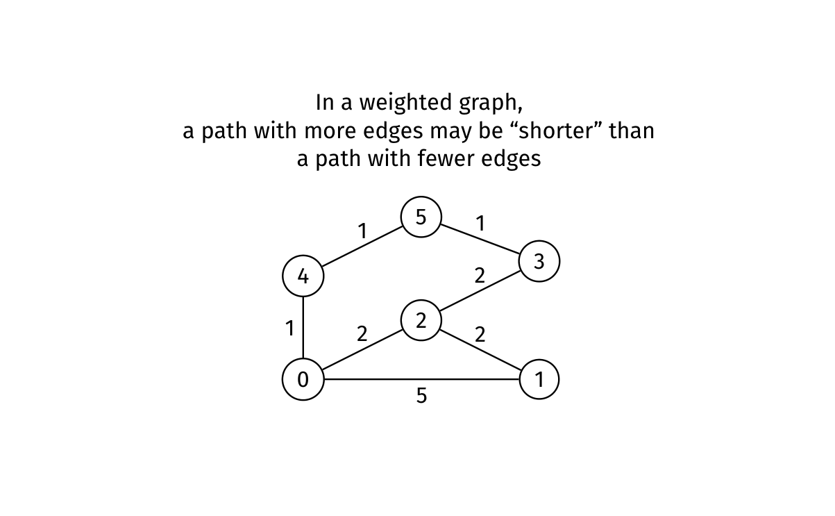
From 0 to 3 in the image, route has three edges of weight 1, total 3. The two-edge route costs . BFS would prefer the latter by hop count; weighted shortest paths need a different method.
Dijkstra's Algorithm#
Preconditions, State and Relaxation#
Dijkstra finds single-source shortest paths when all weights are non-negative. It works for directed or undirected graphs. Zero weights are allowed; negative weights invalidate its greedy finalisation argument.
Maintain dist[v], the cost of the best route currently known from the source to , initially infinity except source distance 0; pred[v], that route's predecessor, initially -1; and a set of unsettled vertices. To settle a vertex means to establish that its current distance is final.
Repeatedly choose the unsettled vertex with smallest distance, settle it, and try its outgoing edges. Relaxing edge means comparing the current dist[w] with a candidate route using :
If candidate is strictly smaller, set dist[w]=candidate and pred[w]=v. A predecessor can change several times while its vertex remains unsettled. Unlike BFS, the first discovered weighted route need not be cheapest.
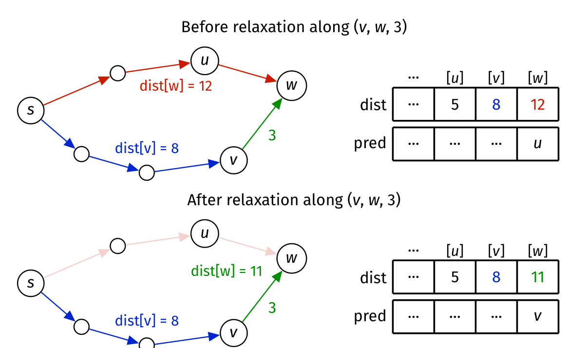
Here dist[v]=8 and edge weighs 3. The candidate cost is 11, improving the old cost 12, so change both distance and predecessor. If the edge instead weighed 6, candidate 14 would not improve 12. Equality need not replace the existing predecessor; there can be multiple shortest paths.
The Lecture's Six-Vertex Trace#
The graph is undirected, with edges , , , , , , , , . Start at 0.
| Vertex settled | Important relaxation decisions | Distances to 0,1,2,3,4,5 afterwards |
|---|---|---|
| Initialisation | Source alone has a known route | |
| 0 | Direct neighbours get costs 14,9,7 | |
| 3 | does not beat 9; reaches 5 | |
| 2 | improves 1; improves 5 | |
| 5 | reaches 4 | |
| 1 | improves 4 | |
| 4 | No remaining improvement |
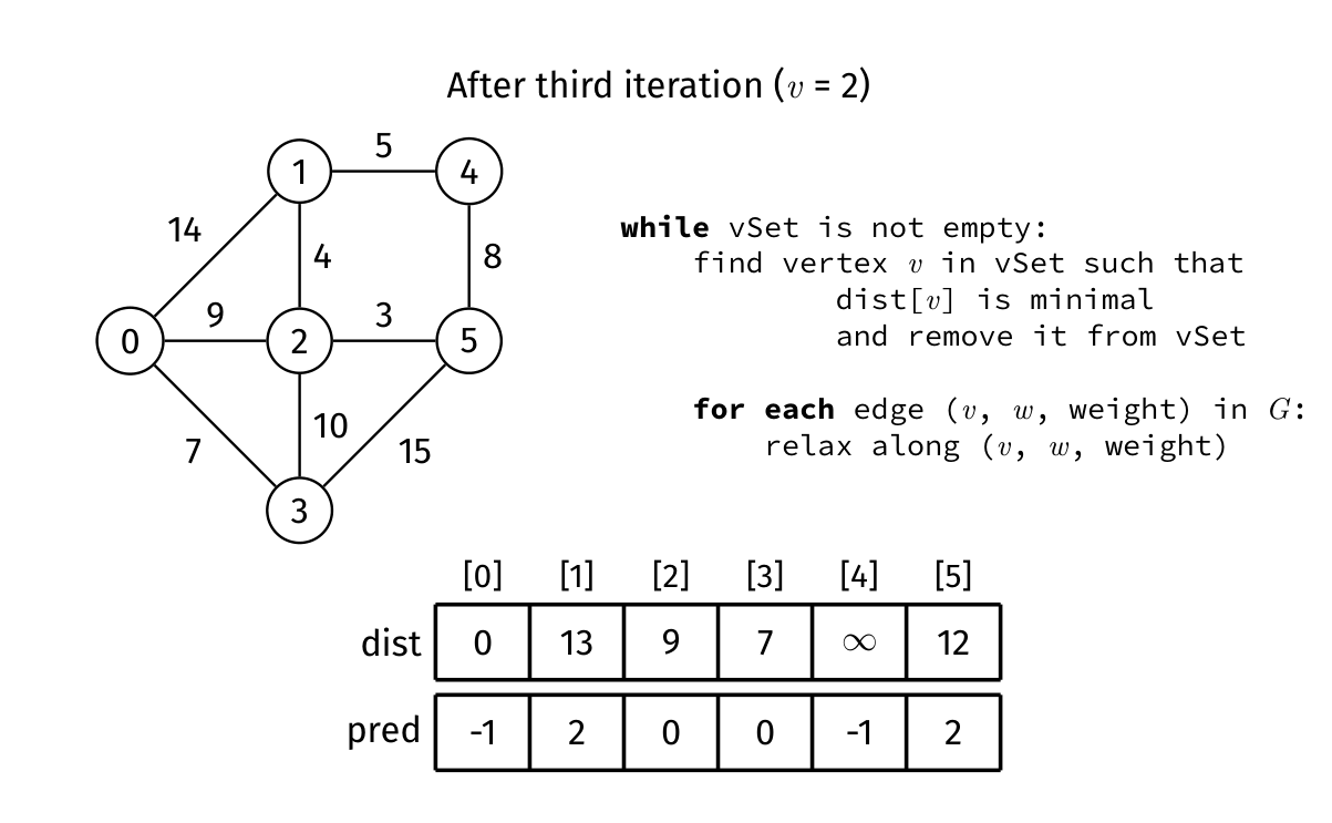
Notice that vertex 5 first has cost 22, then 12. Vertex 1 similarly changes from 14 to 13. Settling order follows tentative distance, not vertex number and not the order that vertices were first discovered.
Vertices: 0, 1, 2, 3, 4, 5. Shortest paths complete; predecessor links reconstruct each reachable path from the start. Enable JavaScript to inspect each step.
The built-in chooses the smallest unsettled distance by a linear scan, matching the lecture's Boolean-set implementation. On equal distances it uses vertex declaration order. The trace relaxes even edges to settled vertices; with non-negative weights they cannot strictly improve an already final distance. Our C implementation skips them explicitly.
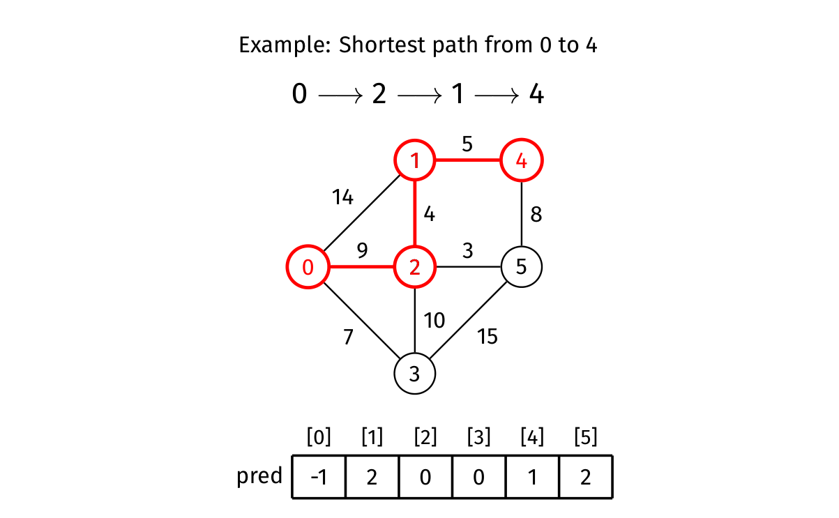
Final predecessors are [-1,2,0,0,1,2]. To recover the route to 4, walk and reverse it. Cost is . The cheaper route to 5 costs 12, but extending it to 4 gives 20, which is worse. A result from source 0 does not generally answer a shortest-path query from 3 to 4: rerun from 3 or use an all-pairs algorithm.
Practice. After settling 2, should vertex 1 of distance 13 be settled before vertex 5 of distance 12 because 1 was discovered earlier?
Note
- Answer
No. Dijkstra selects minimum current distance, so 5 is next. Discovery order is irrelevant. Settling 5 produces a tentative cost 20 for 4; settling 1 later improves it to 18 before 4 is finalised.
Why Settling the Minimum Is Safe#
The invariant has two parts: settled vertices have their true shortest distances; unsettled vertices have the best routes known through already settled intermediate vertices. Each finite tentative distance represents an actual route, so it never underestimates the real shortest distance.
Take minimum unsettled vertex . Suppose a shorter route to it existed. Follow that route from the source to its first unsettled vertex . Its preceding vertex was settled, so relaxing that boundary edge already gave a distance no greater than the cost of the route's prefix to . Since remaining edges have non-negative weights, the prefix costs no more than the whole proposed shorter route to . Therefore dist[x] < dist[v], contradicting that was the minimum unsettled choice. So settling is safe.
Relaxing its outgoing edges then adds exactly the newly permitted routes through , preserving the second part of the invariant. Repeat until all reachable vertices are settled. If the smallest remaining distance is infinity, no remaining vertex is reachable, and we can stop.
The slide proof illustrates the settled/unsettled boundary. Zero-cost suffixes require a non-strict prefix inequality; the contradiction is with the assumed strictly shorter whole route, so zero weights remain valid.
A Complete Scan-Based C Implementation#
This code follows the linear-selection variant. It represents absence with -1, so zero-weight edges remain valid. Weights are non-negative int values; distances use long long. With at most 32 vertices, a simple shortest path has at most 31 edges, so even INT_MAX weights fit safely in long long. We never add to the infinity sentinel.
// Initialize every occupied w[v][u] cell to -1 before inserting edges.
// An undirected edge requires assigning both w[v][u] and w[u][v].
typedef struct {
    int n;
    int w[MAXV][MAXV]; // -1 absent; 0..INT_MAX is a legal weight
} WeightedGraph;

void dijkstra(const WeightedGraph *g, int src,
              long long dist[], int pred[]) {
    assert(g->n > 0 && g->n <= MAXV && src >= 0 && src < g->n);
    bool settled[MAXV] = {false};
    for (int v = 0; v < g->n; v++) {
        dist[v] = LLONG_MAX;
        pred[v] = -1;
        for (int w = 0; w < g->n; w++) assert(g->w[v][w] >= -1);
    }
    dist[src] = 0;
    for (int iteration = 0; iteration < g->n; iteration++) {
        int v = -1;
        for (int x = 0; x < g->n; x++)
            if (!settled[x] && (v == -1 || dist[x] < dist[v])) v = x;
        if (v == -1 || dist[v] == LLONG_MAX) break;
        settled[v] = true;
        for (int w = 0; w < g->n; w++) {
            if (settled[w] || g->w[v][w] == -1) continue;
            long long candidate = dist[v] + g->w[v][w];
            if (candidate < dist[w]) {
                dist[w] = candidate;
                pred[w] = v;
            }
        }
    }
}
pred[src] remains -1 here, as in the lecture, because settled has a separate role and discovery is not encoded by predecessors. Recover a route by stopping at src, not by demanding a self-predecessor. Test dist[dest] != LLONG_MAX before recovery. A zero-edge route from src to itself has cost 0.
For each of at most iterations, minimum selection scans vertices and the matrix scans possible neighbours. Therefore this implementation has time and auxiliary storage, excluding graph and returned arrays. With adjacency lists plus linear minimum selection, scanning actual edges contributes , yielding for simple graphs. Lists alone do not remove the quadratic minimum-selection work.
Practice. Why is LLONG_MAX + weight never evaluated? What result is retained for an isolated non-source vertex?
Note
- Answer
The algorithm breaks when the selected minimum is LLONG_MAX, before scanning its edges. Finite distances can therefore be safely extended. An isolated non-source vertex keeps distance LLONG_MAX and predecessor -1, representing unreachable rather than a very expensive route.
Priority Queues and the Lecture's Cost Shorthand#
A priority queue retrieves the item of highest priority; for Dijkstra, smaller distance means higher priority. A heap can avoid scanning all unsettled vertices, but relaxing an edge also changes that vertex's priority. That update must be counted.
With an indexed binary heap supporting decrease-key in , at most minimum removals and up to distance improvements give time with adjacency lists. A lazy alternative inserts another (distance,vertex) entry after an improvement and skips obsolete entries when popped; it uses potentially queued entries and logarithms of heap size. Both are implementable approaches, but they differ from the scan-based code and trace above. See 19. Priority Queues and Heaps.
The slide's priority-queue row gives by adding edge scanning and minimum removals. That bound also requires cheap priority improvements, obtained amortised by a Fibonacci heap: amortised means a bound on the total cost across a sequence, allowing some individual operations to cost more. A standard binary heap must account for improvements too. Distinguishing these implementations explains the apparent discrepancy rather than changing the lecture's scan variant.
More exam-style practice#
Work each prompt before opening its answer. State the invariant or cost assumption that makes your reasoning valid.
Question 1. Warshall’s algorithm considers intermediate vertex k. If reach[i][k] and reach[k][j] are true, what update is made, and why does the order of k matter to the invariant?
Note
- Answer
Set reach[i][j] to true. After iteration k, the table represents paths whose intermediate vertices come from the processed set through k. The outer loop over k expands that allowed set one vertex at a time.
Question 2. Run one Dijkstra relaxation from settled u with dist[u]=7, edge weight u→v=4, and old dist[v]=15. What changes?
Note
- Answer
The candidate is 7+4=11, so set dist[v]=11 and pred[v]=u. Relaxation alone does not settle v; it remains a frontier candidate until it is the minimum unsettled distance.
Question 3. Kahn’s algorithm processes only 4 of 6 vertices before its zero-indegree queue empties. What has been proved?
Note
- Answer
The remaining directed subgraph contains a cycle, so no topological ordering of all 6 vertices exists. If it were acyclic, some remaining vertex would have indegree zero. The four emitted vertices form only a partial order.
Question 4. Give a three-vertex negative-edge example showing why ordinary Dijkstra’s settled-vertex rule is unsafe.
Note
- Answer
Use s→a=2, s→b=5, b→a=-4. Dijkstra may settle a at 2 before b, but the path s→b→a costs 1. Once a is declared final, later negative relaxation contradicts the rule. Negative edges require another algorithm or stronger preconditions.
Note
Checkpoint
Dijkstra repeatedly settles the smallest tentative distance, then relaxes outgoing edges. Non-negative weights make finalisation safe. A predecessor can change before settlement. Linear minimum selection costs quadratic time; heap bounds depend on both removal and priority-update operations.
Negative Weights and Other Shortest-Path Algorithms#
A negative edge can break Dijkstra even with no negative cycle. Take , , . Dijkstra settles A at 2 before B, yet the route costs 1. The proof failed because the prefix to B costs 5, more than the eventual route cost 1: a negative suffix invalidates its non-negative-prefix argument.
A negative cycle has total edge weight below zero. If it is reachable from a source and can lead to a destination, repeatedly going around it makes route costs arbitrarily small. There is then no finite minimum for that source-destination pair. An unreachable negative cycle does not affect a source's reachable shortest paths. In an undirected graph, a negative edge allows repeated out-and-back travel with negative cost, so unrestricted-walk shortest paths are especially problematic.
The slides name these alternatives for curiosity:
- Bellman–Ford solves single-source shortest paths with negative edges and detects reachable negative cycles. Repeatedly relax all edges for up to passes. A shortest route without a negative cycle can be made simple and use at most edges. A further improvement after those passes indicates a reachable negative cycle. Its usual worst-case time is , with distance/predecessor storage.
- Floyd–Warshall solves all-pairs shortest paths by allowing intermediate vertices as Warshall does, but uses minimum and addition instead of Boolean OR and AND. Its recurrence is . It costs time and result storage. Negative edges are allowed; finite shortest routes require no relevant negative cycle. A negative diagonal after processing detects a negative cycle.
These are distinct from Boolean Warshall, which computes route existence rather than cost. Floyd–Warshall normally initialises distance to self as 0, preserves the least direct edge cost, and uses infinity for absent routes.
The following supplementary Bellman–Ford example has a negative edge but no cycle. Watch A improve from 2 to 1 when the edge from B is processed; it is not permanently settled after its first distance.
Vertices: S, A, B. Shortest paths complete; predecessor links reconstruct each reachable path from the start. Enable JavaScript to inspect each step.
Practice. Is a negative edge alone sufficient to say no shortest path exists?
Note
- Answer
No. In the directed acyclic example above, the finite shortest route from S to A has cost 1. The obstruction to finite unrestricted-route minima is a relevant negative cycle, not merely a negative edge. Dijkstra still cannot be used with arbitrary negative edges because its finalisation rule can fail.