06. Divide and Conquer Sorting
Divide, Solve, Combine#
Divide and conquer splits a problem into smaller problems, solves them, and combines their solutions. Merge sort divides by position before solving; quicksort divides by comparison with a pivot. Both recurse, but their guarantees depend on different mechanisms.
The lecture C uses inclusive [lo,hi] ranges. A one-item or empty range satisfies lo >= hi and is already sorted. Splitting an array means passing index ranges over the same storage, not necessarily allocating two copied input arrays.
Merge Sort: Sort Halves, Then Merge#
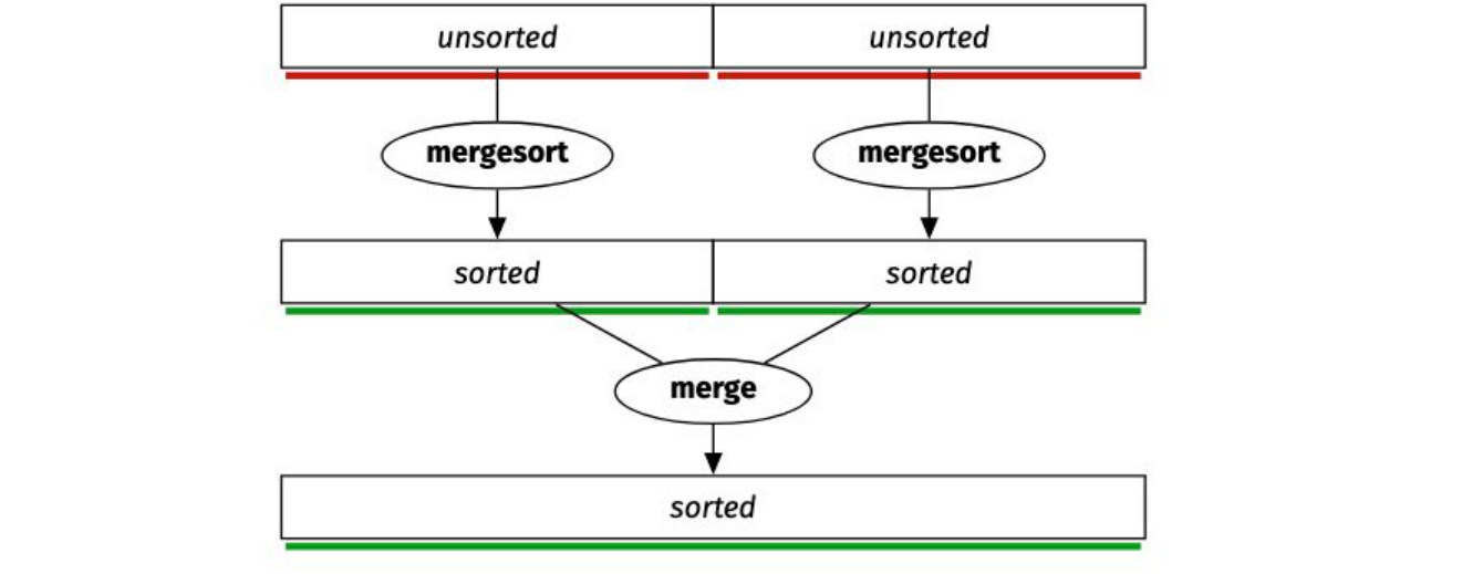
Each recursive call promises a sorted half. Merging can then compare only each half's next unused element, because that element is its smallest remaining one. This is the whole point of sorting the halves first: the combine step can be linear rather than searching repeatedly for global minima.
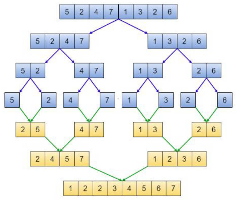
Read the blue arrows downward as recursive splitting and the lower rows upward as returned sorted ranges. Eight entries give three split levels. Every item participates in one merge per merge level, giving linear work across the entire level.
Trace a Merge and Preserve Ties#
Merge the lecture's sorted halves [2_A,4,5,7] and [1,2_B,3,6]:
| Heads available | Choose | Why | Output so far |
|---|---|---|---|
2_A, 1 |
1 | Smaller right head | [1] |
2_A, 2_B |
2_A |
Equal: take left | [1,2_A] |
4, 2_B |
2_B |
Smaller right head | [1,2_A,2_B] |
| 4, 3 | 3 | Smaller right head | [1,2_A,2_B,3] |
| 4, 6 | 4 | Smaller left head | [1,2_A,2_B,3,4] |
| 5, 6 | 5 | Smaller left head | [1,2_A,2_B,3,4,5] |
| 7, 6 | 6 | Smaller right head | [1,2_A,2_B,3,4,5,6] |
| 7, exhausted | 7 | Only left remains | [1,2_A,2_B,3,4,5,6,7] |
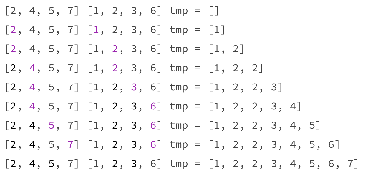
The output invariant is that the temporary prefix is sorted and contains exactly the smallest consumed entries. Choosing the smaller head is safe because no later element in its sorted half is smaller. Taking the left head on equality preserves cross-half tie order; recursive stability preserves order within each half. Together these establish the whole sort's stability.
C Implementation With One Shared Buffer#
tmp must point to a buffer of at least n integers, separate from the input. These functions are an integer specialisation of the lecture mechanism:
static void merge(int a[], int tmp[], int lo, int mid, int hi) {
    int i = lo, j = mid + 1, k = lo;
    while (i <= mid && j <= hi) {
        if (a[i] <= a[j]) tmp[k++] = a[i++];
        else tmp[k++] = a[j++];
    }
    while (i <= mid) tmp[k++] = a[i++];
    while (j <= hi) tmp[k++] = a[j++];
    for (k = lo; k <= hi; k++) a[k] = tmp[k];
}

void mergeSort(int a[], int tmp[], int lo, int hi) {
    if (lo >= hi) return;
    int mid = lo + (hi - lo) / 2;
    mergeSort(a, tmp, lo, mid);
    mergeSort(a, tmp, mid + 1, hi);
    merge(a, tmp, lo, mid, hi);
}
Copying back only after both halves are consumed prevents overwriting unread input. Sharing a buffer avoids allocating a full buffer at every active call. Allocate it once in the caller, check allocation, call mergeSort(a,tmp,0,n-1), then free it. The same helpers work for bottom-up merges described below.
Watch the singleton ranges combine, then compare the two equal twos at the final merge. The player's merge ranges use exclusive upper bounds internally; its representation differs in index convention, but its stable merge decisions match this lesson.
Values: 5, 2, 4, 7, 1, 3, 2, 6. Sorting complete: every adjacent pair is in ascending order. Final values: 1, 2, 2, 3, 4, 5, 6, 7. Enable JavaScript to inspect each step.
Practice. Merge [1,2,3] with [4,5,6]. How many key comparisons are needed, and how many items are copied to the buffer?
Note
- Answer
Compare 1,2,3 with the right head 4, making three comparisons. The left half then exhausts, so append the remaining three without further key comparisons. Six items still go into the buffer and six are copied back. Linear merge work does not mean exactly n key comparisons on every input.
Derive Time and Space#
For n total items in a merge, at most n-1 head comparisons occur; buffer writes and copy-back both process n items. Merge work is Θ(n). Recursion has logarithmically many levels, and all merges on one level collectively process n items: Θ(n log n) total in best, average and worst cases for this implementation. It does not skip a merge because two halves happen already to be in order.
The shared buffer uses Θ(n) auxiliary storage. Recursive frames add Θ(log n) maximum depth, so total auxiliary space remains linear. Splitting by indices costs constant work per call; it is merging, not physically copying two halves at every split, that creates the linear level work.
Bottom-Up Merge Sort#
An iterative alternative starts with sorted runs of length one. Merge adjacent pairs to produce length-two runs, then length-four, then length-eight, until one run covers the array. On ten items, the final pair at some levels can be shorter than the nominal width; clamp both boundaries to the real end.
width = 1
while width < n:
    for lo = 0, 2*width, 4*width, ... below n:
        mid = min(lo + width - 1, n - 1)
        hi  = min(lo + 2*width - 1, n - 1)
        if mid < hi: merge the two ranges
    double width
Here is the actual inclusive-index C loop, reusing the merge helper above. The outer width m describes runs already sorted before that pass. hi - m ensures a full left run exists before asking for a right run; end clamps a short final right run.
void mergeSortBottomUp(int a[], int tmp[], int lo, int hi) {
    if (lo >= hi) return;
    for (int m = 1; m <= hi - lo; ) {
        for (int i = lo; i <= hi - m; ) {
            int rightAvailable = hi - (i + m) + 1;
            int rightLength = rightAvailable < m ? rightAvailable : m;
            int end = i + m + rightLength - 1;
            merge(a, tmp, i, i + m - 1, end);
            if (rightAvailable <= m) break;
            i += 2 * m;
        }
        if (m > (hi - lo) / 2) break;
        m *= 2;
    }
}
For exam tracing, the simpler width pseudocode is usually clearer; the guarded C arithmetic only prevents overflowing a signed int near its limit. Both forms use Θ(n) work at each of Θ(log n) passes, Θ(n) shared-buffer space, and no recursive stack. A pass can include one short unpaired run, which is already sorted and is carried into the next pass.
Note
Checkpoint
Sorted halves make merging linear. A left-on-equality choice gives stability. Linear work per level across logarithmically many levels gives linearithmic total time; the buffer makes array merge sort non-in-place.
Quicksort: Partition Around a Pivot#
A pivot is a chosen item used to divide the range. A partition rearranges the other items so values at most the pivot lie on one side and values at least it on the other, then places the pivot between them. Neither side is necessarily internally sorted. Recursively sorting the sides completes the job, with no final merge.
The lecture's first option chooses a[lo] and scans inward from both ends. This differs from the site's built-in last-pivot Lomuto implementation. We use the lecture code and an authored trace, rather than quietly changing the partition rule.
int partition(int a[], int lo, int hi) {
    int pivot = a[lo];
    int l = lo + 1, r = hi;
    while (1) {
        while (l <= r && a[l] <= pivot) l++;
        while (l <= r && a[r] >= pivot) r--;
        if (l > r) break;
        swap(a, l, r);
    }
    swap(a, lo, r);
    return r;
}

void quickSort(int a[], int lo, int hi) {
    if (lo >= hi) return;
    int p = partition(a, lo, hi);
    quickSort(a, lo, p - 1);
    quickSort(a, p + 1, hi);
}
Within the active range, indices already passed on the left hold values <= pivot; indices already passed on the right hold values >= pivot. The stopped pair has a large value on the left and a small value on the right, so exchanging it repairs both placements. Even though the code does not explicitly increment after swapping, the next scans consume the exchanged values. At crossing, r is the last left-side position; exchanging a[lo] with a[r] puts the pivot in its final sorted position.
The Lecture Partition, Step by Step#
For [50,34,123,65,12,78,89,23,54,3], the pivot is 50. The left scan passes 34 and stops at 123; the right scan immediately stops at 3. Swap them. Next the left scan passes the exchanged 3 and stops at 65; the right scan passes 123 and 54, stopping at 23. Swap them. Then the left scan passes 23 and 12, stopping at 78. The right scan passes 65,89,78 and crosses. Finally swap the pivot with 12 at index four.
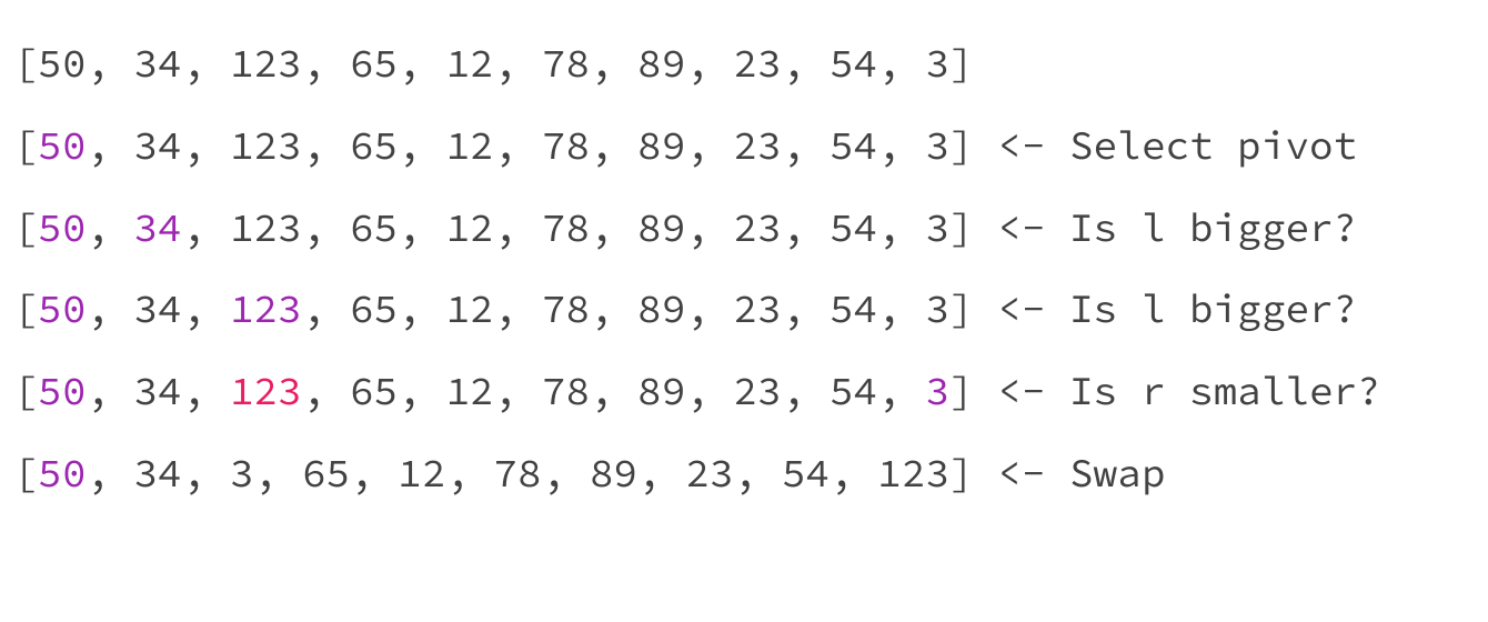
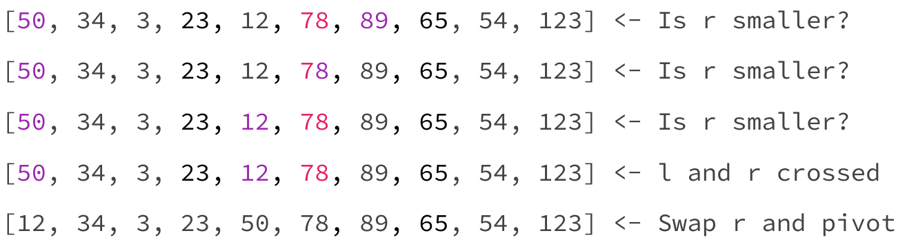
This custom player starts with the lecture partition and continues through every recursive range to the sorted result. Its code tab contains the C routine below; the complexity panel derives the case bounds from partition work and recursion depth. Follow the active range and pivot index: a pivot is finished, but its two sides are not, until recursion returns. The first partition uses the lecture values and decisions exactly.
Values: 50, 34, 123, 65, 12, 78, 89, 23, 54, 3. Every pivot is in its final position and every singleton returned: the whole array is sorted. Final values: 3, 12, 23, 34, 50, 54, 65, 78, 89, 123. Enable JavaScript to inspect each step.
The first partition result is [12,34,3,23,50,78,89,65,54,123]. The next left partition chooses 12, exchanges 34 and 3, and places 12 at index 1. The local pair [34,23] then becomes [23,34]. On the right, pivot 78 leads to [65,54,78,89,123]; the two remaining pairs finish as [54,65] and [89,123]. The complete result is [3,12,23,34,50,54,65,78,89,123]. These recursive calls are part of sorting; stopping after the first partition would leave both sides disordered.
Practice. Why do the recursive calls exclude p? Why can't partition claim the left side is already sorted?
Note
- Answer
The pivot is already between all values that may precede and follow it, so its final rank is established and including it again risks failing to shrink a subproblem. Partition only establishes a relation to the pivot. Values like [12,34,3,23] all belong left of 50 but remain internally unordered.
The Second Partition Option#
The slides also give a meeting-index version using l < r. It stops scans when the indices meet and checks the meeting value before choosing the pivot destination. If that value is larger than the pivot, decrement the meeting index, then exchange the pivot there. This final check substitutes for the first option's crossing logic. The two versions use different stopping conditions; do not mix l < r scans with an unmodified r pivot placement borrowed from the crossing version.
For [2,1], the meeting index starts at the second entry; since that value is smaller than 2, swap the pivot into index one. For [1,2], the meeting value is larger, so move the pivot destination back to index zero. These tiny cases explain why the final adjustment is necessary.
The actual option-two C helper is worth keeping separate. It uses the same swap helper as option one, but its loop stops at a meeting index rather than after crossing:
int partitionMeet(int a[], int lo, int hi) {
    int pivot = a[lo];
    int l = lo + 1, r = hi;
    while (l < r) {
        while (l < r && a[l] <= pivot) l++;
        while (l < r && a[r] >= pivot) r--;
        if (l == r) break;
        swap(a, l, r);
    }
    if (pivot < a[l]) l--;
    swap(a, lo, l);
    return l;
}

void quickSortMeet(int a[], int lo, int hi) {
    if (lo >= hi) return;
    int p = partitionMeet(a, lo, hi);
    quickSortMeet(a, lo, p - 1);
    quickSortMeet(a, p + 1, hi);
}
For [5,3,7,2,1,4,6,8], l passes 3 and stops at 7; r passes 8,6 and stops at 4. Exchange 7,4 to obtain [5,3,4,2,1,7,6,8]. The scans then meet at index 5, whose value 7 exceeds pivot 5; decrement the destination to 4 and place 5 there. The result [1,3,4,2,5,7,6,8] has the same partition property as option one, but the final index comes from a different stopping rule.
Values: 5, 3, 7, 2, 1, 4, 6, 8. Swap 5 with a[4]=1. Result 1,3,4,2,5,7,6,8 has pivot 5 at final index 4; both sides remain unsorted. Final values: 1, 3, 4, 2, 5, 7, 6, 8. Enable JavaScript to inspect each step.
One partition still makes only monotone scans through at most n entries: Θ(n) time and Θ(1) working variables. Calling it recursively under quickSort yields the balanced Θ(n log n) / extreme Θ(n²) cases and corresponding Θ(log n) / Θ(n) stack depths shown in the player. Do not infer that either partition is stable; long-range exchanges can reverse equal-key records.
Practice. In option two, why is the last if (pivot < a[l]) l--; needed on [1,2], but not [2,1]?
Note
- Answer
On [1,2], meeting value 2 is greater than pivot 1, so l moves back to index zero; the pivot remains at index zero. On [2,1], meeting value 1 belongs left, so no decrement is needed and the pivot swaps to index one. Without the conditional, [1,2] would incorrectly place pivot 1 after 2.
Derive Costs and Duplicate Behaviour#
One partition advances two scans across the range, so its work is linear. Balanced pivot ranks give T(n)=2T(n/2)+Θ(n), hence linearithmic time and logarithmic active depth. If the pivot is always an extreme, subproblem sizes are zero and n-1; summing shrinking linear partitions gives quadratic time and linear recursive depth.
For uniformly random permutations of distinct keys, the expected partition ranks yield Θ(n log n) time. This is a distribution-dependent statement. Random pivot selection can instead provide an expectation over random choices on a fixed distinct-key input. Worst-case time remains quadratic.
With the lecture's <= and >= scan rules, an all-equal input is especially revealing: the left scan consumes the range, and the pivot ends at the last position. The remaining recursive range has size n-1, so equal input can still be quadratic, even with random pivot selection or median-of-three. A three-way partition would handle ties differently, but that is an additional variant, not the code taught here.
Partition uses constant working variables and no merge buffer. The ordinary recursive implementation still needs logarithmic expected or linear worst-case stack space. Its long-distance exchanges are unstable. Already sorted input makes a fixed first pivot poor rather than accelerating the sort, so it is non-adaptive.
Practice. Partition [4,4,4,4] with the first option. Where does the pivot go, and what is the next nonempty recursive range?
Note
- Answer
The left scan consumes indices 1,2,3 and becomes 4. The right scan does not run because l > r. Exchange indices 0 and 3, leaving equal values unchanged; return 3. Recursion continues on indices 0 through 2, so the same degenerate split repeats.
Improve Pivot Choice and Small Ranges#
Median of Three#
Inspect lo, midpoint and hi, then put their median at lo for the same partition helper. The lecture deliberately arranges a[mid] <= a[lo] <= a[hi]; it does not simply leave all three samples in index order.
void medianOfThree(int a[], int lo, int hi) {
    int mid = lo + (hi - lo) / 2;
    if (a[mid] > a[lo]) swap(a, mid, lo);
    if (a[lo] > a[hi]) swap(a, lo, hi);
    if (a[mid] > a[lo]) swap(a, mid, lo);
}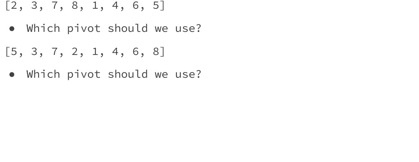
For [2,3,7,8,1,4,6,5], sample values are 2,8,5. The helper transforms the array to [5,3,7,2,1,4,6,8]; the pivot is 5. This avoids extreme pivots on many ordered distinct inputs. It does not prove every partition is balanced and does not eliminate the quadratic worst case.
The three comparisons above order only the sampled positions, not the whole range. The recursive variant uses the same first-pivot partition after installing the sample median at lo:
void quickSortMedian(int a[], int lo, int hi) {
    if (lo >= hi) return;
    medianOfThree(a, lo, hi);
    int p = partition(a, lo, hi);
    quickSortMedian(a, lo, p - 1);
    quickSortMedian(a, p + 1, hi);
}
The player shows the three sample positions, their exact exchanges, the subsequent partition, and the still-unsorted recursive ranges. Read its C tab alongside the steps.
Values: 2, 3, 7, 8, 1, 4, 6, 5. Continue with lo..3 and 5..hi, re-sampling lo, midpoint and hi separately inside each recursive call. Final values: 1, 3, 4, 2, 5, 7, 6, 8. Enable JavaScript to inspect each step.
On the eight-item example, the sample is 2,8,5; its median is 5, not the true median of all eight items. After partition, the pivot is at index four in [1,3,4,2,5,7,6,8]. This is a better pivot than original first element 2 on this particular input, but neither side is fully sorted. At each recursive call, sample that call's lo, midpoint and hi again. On equal keys all three samples may be equal, and this two-way partition still degenerates.
Practice. Does median-of-three change the worst-case class or guarantee that each side has half the items?
Note
- Answer
No. It inspects only three positions. An adversarial arrangement can still make their median an extreme rank among the complete range, causing a size n-1 side repeatedly. It improves many ordinary inputs but leaves Θ(n²) worst-case time and Θ(n) worst-case active stack depth.
Random Pivot#
Choose an index in [lo,hi], exchange it with lo, then call the same helper. In C, srand(seed) seeds the generator once, such as in main; rand() obtains a generated number. The deck's int i = srand() % ... is a typo: srand requires an argument and returns no number.
A complete recursive form makes the generator's role unambiguous. randomIndex is an illustrative implementation for modest int ranges; assume the span is positive, fits int, and is no greater than the generator's output span. The % operation can bias choices. A theorem that assumes uniformly chosen ranks uses an unbiased generator or a suitable rejection-sampling helper.
#include <stdlib.h>

int randomIndex(int lo, int hi) {
    return lo + rand() % (hi - lo + 1);
}

void quickSortRandom(int a[], int lo, int hi) {
    if (lo >= hi) return;
    swap(a, lo, randomIndex(lo, hi));
    int p = partition(a, lo, hi);
    quickSortRandom(a, lo, p - 1);
    quickSortRandom(a, p + 1, hi);
}
For an exam hand trace, state the chosen random index; the algorithm has no unique deterministic trace without it. This player fixes one illustrative draw, index 6, then follows all scan/exchange decisions for that partition. The code tab shows the recursive routine and the complexity panel separates expectation from worst case.
Values: 2, 3, 7, 8, 1, 4, 6, 5. Recursive calls choose fresh random indices independently; this one draw does not force later balanced splits. Final values: 4, 3, 5, 2, 1, 6, 8, 7. Enable JavaScript to inspect each step.
The partition itself remains Θ(n) regardless of how its pivot was selected. With a uniform random rank on a fixed distinct-key input, expected recursion work is Θ(n log n); with a possible run of extreme ranks, worst-case work is still Θ(n²). If all keys are equal, the lecture's inclusive <= and >= scans place each pivot at an end no matter which equal index was sampled. Randomness cannot cure this duplicate-specific chain; three-way partitioning would group equal keys into a middle region in one pass, but that is beyond the two partition helpers in this deck.
Insertion-Sort Cutoff#
For small fixed-size ranges, call insertion sort instead of creating more recursive partition calls. Use the same index convention: the elementary insertion routine takes inclusive lo,hi.
The slide combines a fixed insertion cutoff with median-of-three. Here hi-lo < 5 means at most five entries; empty or singleton ranges also satisfy the guard. The snippet reuses insertionSort from Elementary Sorting and the helpers already shown in this chapter.
#define THRESHOLD 5

void quickSortHybrid(int a[], int lo, int hi) {
    if (lo >= hi) return;
    if (hi - lo < THRESHOLD) {
        insertionSort(a, lo, hi);
        return;
    }
    medianOfThree(a, lo, hi);
    int p = partition(a, lo, hi);
    quickSortHybrid(a, lo, p - 1);
    quickSortHybrid(a, p + 1, hi);
}
The hybrid player follows one large range through sample ordering and partition, then shows insertion sort finishing both small recursive ranges. Its C tab and per-case derivations refer to this exact fixed-threshold variant.
Values: 2, 3, 7, 8, 1, 4, 6, 5. Insert 6 before 7; 8 stays. The complete array is 1,2,3,4,5,6,7,8. Final values: 1, 2, 3, 4, 5, 6, 7, 8. Enable JavaScript to inspect each step.
For a fixed cutoff k, insertion takes at most O(k²) work per leaf, and there are at most O(n) such constant-size leaves. Their aggregate is O(n) when k is a fixed constant; larger quicksort partition levels still determine Θ(n log n) balanced/expected work and Θ(n²) worst work. If k grew with n, that constant-size argument would no longer apply. The cutoff reduces call overhead but does not make the routine stable: the large-range partition can still reverse equal items.
Practice. On the player input of eight values with THRESHOLD=5, why does the first call partition but the two resulting ranges use insertion sort?
Note
- Answer
The initial inclusive range [0,7] has hi-lo=7, so the cutoff test is false. After the median pivot 5 settles at index four, the sides [0,3] and [5,7] have differences 3 and 2, both below 5. Each side is insertion-sorted in place; pivot index four is excluded.
Practice. Which would you choose to preserve zID order among equal marks: ordinary quicksort or stable merge sort? What if an embedded system has too little memory for a linear buffer?
Note
- Answer
Stable merge sort preserves the established tie order; ordinary quicksort cannot promise it. A constrained system may favour an array-in-place alternative, but quicksort's worst stack depth must still be addressed. Heapsort offers constant auxiliary space and a worst-case linearithmic guarantee, with an unstable result. The best choice depends on both output requirements and memory.
More exam-style practice#
Work each prompt before opening its answer. State the invariant or cost assumption that makes your reasoning valid.
Question 1. Merge [2a,5] and [2b,3] by key while preserving stability. What order should the equal 2 records have, and which merge comparison makes that happen?
Note
- Answer
The merged order is 2a,2b,3,5. On equal keys choose the item from the left run first, for example by testing left.key <= right.key. Choosing the right on equality would reverse records that were ordered across the two halves.
Question 2. Quicksort repeatedly chooses the first element as pivot on an already sorted length-n array. Write the recurrence and explain the resulting depth.
Note
- Answer
Each partition places the pivot at one end, leaving a subproblem of size n-1: T(n)=T(n-1)+Θ(n)=Θ(n²). The recursive chain has depth Θ(n), so a straightforward recursive implementation also uses Θ(n) stack space.
Question 3. For keys [1,2,3,4,5,6,7], compare first-element and median-of-three pivot selection on the initial partition. Does median-of-three guarantee good splits later?
Note
- Answer
First-element selection uses 1 and yields a 0/6 split; median of first, middle and last chooses 4 and yields a 3/3 split initially. Median-of-three is a heuristic using three samples. Later partitions can still be badly unbalanced, so its worst-case time remains Θ(n²).
Question 4. Why does replacing tiny quicksort subproblems with insertion sort often help without changing average asymptotic time?
Note
- Answer
Insertion sort has small constant overhead and runs on short, often partly ordered ranges. With a fixed cutoff k, each leaf costs at most O(k²), while partitioning across balanced levels remains Θ(n log n) on average. The cutoff changes constants, not the general worst-case possibility of bad partitions.
Note
Checkpoint
Merge sort guarantees balanced positional splits and pays for a buffer. Quicksort avoids that buffer but depends on pivot ranks and partition rules. The slides teach both inward-scan partition stopping rules, median-of-three, random-pivot and fixed insertion-cutoff variants; each changes how a pivot or leaf is handled without making ordinary quicksort stable or removing every worst case.
Which Version Fits the Requirement?#
| Version | Pivot / stopping rule | Typical reason to use it | Important limit |
|---|---|---|---|
| Lecture first option | First value; scans cross | Simple invariant and exact lecture trace | Sorted or all-equal input can form a chain |
| Lecture second option | First value; scans meet, then adjust destination | Same partition guarantee with a different loop boundary | Never mix its meeting rule with option-one final swap |
| Median of three | Median of lo, midpoint, hi moved to lo |
Avoid many bad fixed-first-pivot cases | Three samples do not guarantee a balanced split |
| Random pivot | Sampled index moved to lo |
Expected protection against a fixed adversarial distinct-key order | Possible quadratic run; duplicate degeneration remains |
| Insertion cutoff | Median pivot on large ranges, insertion on small ones | Avoid recursive overhead at small sizes | Fixed cutoff changes constants, not asymptotic worst case |
For records already sorted by zID that must retain zID order among equal marks, choose stable merge sort. The lecture's salary example has the same requirement: equal-salary employees must retain their original hiring order, so an unstable quicksort is unsuitable. If memory is tightly limited, in-place partitioning may help, but ordinary quicksort can use linear stack in its worst case. For almost sorted arrays, a fixed first pivot is a poor choice, while insertion sort can exploit the small inversion count. The deck briefly names Timsort as a further practical hybrid; no Timsort code or complexity contract is part of this lecture. No single sort dominates every requirement.