Vector Spaces

6.1 Definitions and examples of Vector Spaces#

To define a vector space, we need a mathematical system which consists of the following four things:

1. A set $V$ of elements called "vectors".

2. A "vector-addition" rule that combines a pair of vectors from $V$. This is usually just represented by a $+.$ For vectors $\mathbf{v}, \mathbf{w} \in V,$ you combine them by doing $\mathbf{v} + \mathbf{w}.$

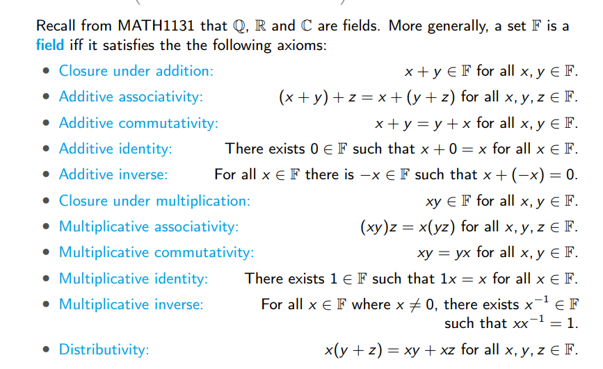
3. A field of scalars, denoted by $\mathbb{F}$, where $\mathbb{F}$ could denote the rational numbers $\mathbb{Q}$ or the real numbers $\mathbb{R}$ or the complex numbers $\mathbb{C}$. There are other less common examples too.
   
   

4. A "multiplication by a scalar" rule for combining a vector from $V$ and a scalar from $\mathbb{F}$ to form a vector. This is probably the most confusing one.

   Basically, from the previous 3 rules, you can discern that a vector can have many possible forms (i.e. made up of only 1s and 0s, or of 2 dimensional matrices etc.), hence, a proper way of determining what happens when scalars multiply such vectors must be formed. There cannot be a default way for every vector as its contents may or may not be different per vector type.

   If $\lambda$ is a scalar and $\mathbf{v}$ is an element of $V$, then $\lambda * \mathbf{v}$ means the result of multiplying $\mathbf{v}$ by the scalar $\lambda$.

   You can internalise this using these examples:

   • Standard Rule: If $V$ is a 2D coordinate space and $\mathbb{F}$ is the real numbers, the rule is $\lambda * (x,y) = (\lambda x, \lambda y)$.
   • Matrix Rule: if $V$ is a set of $2 \times 2$ matrices, multiplying by a scalar means applying it to all four entries inside the matrix grid.
   • Function rule: If $V$ is a set of functions, then multiplying a function $f(x)$ by a scalar $\lambda$ creates a brand new function $g(x)$, defined by the rule $g(x) = \lambda \cdot f(x)$.

The system is then denoted by $(V, +,*, \mathbb{F})$. Often times we can omit the $*$ if its representation remains obvious.

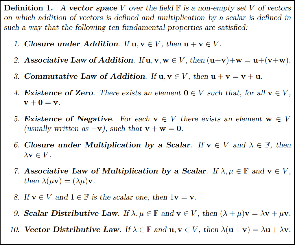
We can now give a formal definition of a vector space.

Note:
1. Each of the basic rules is called an axiom
2. The vector $-\mathbf{v}$ in axiom 5 and the vector formed by multiplying $\mathbf{v}$ with the scalar -1 are not the same by definition.
3. Formally, axiom 7 says $\lambda * (\mu * \mathbf{v}) = (\lambda \mu) * \mathbf{v}$.
4. In axiom 9, the addition on the left is the addition of two scalars while the addition on the right is the addition of two vectors. They are different additions.
5. Two vector spaces are only the same when all the four things are the same $(V, +,*, \mathbb{F})$. However, different vector spaces with the same set of vectors are rarely discussed, unlike different sets of vectors with the same set of scalars and the same operations.
6. When there is no confusion, we shall simply call $(V, +,*, \mathbb{F})$, the vector space $V$.

It is very difficult from the definition alone to acquire a good intuitive understanding - a "gut feeling" - for what is meant by a vector space. You need to supplement the definition by a good “rough idea” of what a vector space is. A good rough idea could be:

A vector space is “something where we know how to add objects and multiply objects by numbers, and where the addition and multiplication satisfy ‘sensible’ laws”

Examples of sets which are vector spaces#

Example 1 (The Vector Space $\mathbb{R}^n$). This represents the set of all vectors of all reals in any $n\text{th}$ dimension.

$$\mathbb{R}^n = \left\{ \mathbf{x} : \mathbf{x} = \begin{pmatrix} x_1 \\ \vdots \\ x_n \end{pmatrix} \text{ for } x_1, \dots, x_n \in \mathbb{R} \right\}.$$

The set of scalars is simply $\mathbb{R}$.
Vector addition is then defined by

$$\begin{pmatrix} x_1 \\ \vdots \\ x_n \end{pmatrix} + \begin{pmatrix} y_1 \\ \vdots \\ x_n \end{pmatrix} = \begin{pmatrix} x_1+y_1 \\ \vdots \\ x_n +y_n\end{pmatrix}.$$

To prove that it is a vector space, it is necessary to show that all ten axioms listed in the definition are satisfied by the system.

All the axioms are general statements about arbitrary vectors and scalars. We have to prove the axioms are satisfied by any:

$$\mathbf{u}=\begin{pmatrix} u_1 \\ \vdots \\ u_n \end{pmatrix}, \mathbf{v} = \begin{pmatrix} v_1 \\ \vdots \\ v_n \end{pmatrix}, \mathbf{w}=\begin{pmatrix} w_1 \\ \vdots \\ w_n \end{pmatrix}, \text{ and } \lambda,\mu \in \mathbb{R}.$$

Lot's of working out to prove all 10 axioms

After we have checked that all ten axioms are satisfied, we can conclude that the system is a vector space, or simply $\mathbb{R}^n$ is a vector space over $\mathbb{R}$.

Example 2 (The Vector Space $\mathbb{C}^n$). The set of vectors similar to example 1 but in the field of the complex numbers.

To prove that this is a vector space it is necessary to show that the ten vector space axioms are satisfied. This proof is formally identical to that for $\mathbb{R}^n$ over $\mathbb{R}$ since only basic operations are involved.

Example 3 (The Vector Space $M_{mn}=M_{mn}(\mathbb{R})$ of Real Matrices). This represents a vector made up of matrices of dimensions $m,n$ where every number inside these matrices must be a real number (the scalar field $\mathbb{F}$ in this case). There is a natural and straightforward generalisation to $M_{mn}(\mathbb{F})$, where the entries come from the field $\mathbb{F}$.

Example 4 (The Vector Space of Polynomials). This is simply the vector space representing every possible polynomial: $x^2, 3x^{21}+3, 12+2x^{765}+9x^{54355}$ etc. However it is worth noting that the set of all real-valued functions on $\mathbb{R}$ can form a vector space, as does the set of all continuous functions (so stuff like $\sin(x)$ or $e^x$). To represent the set of all real polynomials, you write $\mathbb{P}(\mathbb{R})$.

A vector $p \in \mathbb{P}(\mathbb{R})$ is the polynomial given by $p(x) = a_0+a_1x+\dots+a_nx^n=\sum_{k=0}^{n} a_kx^k$.
It is important to note that $p(x)$ is not in considered a vector whilst $p$ is. In other words, $p$ is a real-valued function whilst $p(x)$ is the value of the function at $x$.

One more thing to note is that $\mathbb{P}(\mathbb{R})$ has infinite dimensions since a polynomial can always have a higher leading coefficient since it is in the field of real numbers. You can generalise the field by simply denoting them as $\mathbb{P}(\mathbb{F})$ over a field $\mathbb{F}$. I think any field with addition and multiplication by a scalar similarly defined is also a vector space.

For any non-negative integers $n$, the subset of all polynomial degrees n or less including the zero polynomial is again a vector space.

$$\mathbb{P}_n(\mathbb{F})=\{p:p\text{ is a polynomial over } \mathbb{F}, \text{degree of } p \leq n \text{ or } p=0\}.$$

Examples of sets which are NOT vector spaces#

Example 1 ($\mathbb{Z}^3$, the set of vectors with integer components)
This is simply represented by $(x,y,z)$, and there are 2 axioms that this set breaks.
Since we have not specified the field of these vectors, the default field for scalar's is usually the real numbers $\mathbb{R}$. Looking at Axiom 6, any vector multiplied by any scalar in the field must result in a vector that stays within the original set. However, suppose

$$\lambda = 0.3, \mathbf{v}=(1,2,3)$$

then, $\lambda \mathbf{v} = (0.3,0.6,0.9)$, since this vector consists of at least one non-integer member, it cannot be in the original set, and thus the space is not closed.

Limiting the scalars to only consist of integers $\mathbb{Z}$ fixes our previous problem, however it breaks the very definition of . Since the integers don't have a multiplicative inverse (i.e. there does not exist a number $z$ in the integers such that $z z^-1 = 1$), you cannot choose a field to be integers only.

A vector space is fundamentally designed for continuous scaling; you need to be able to stretch or shrink a vector by any microscopic fraction. Because integers are rigid, whole steps, they can't handle being shrunk by fractions, which ruins the geometry required to be a true vector space.

Example 2 (The set of all matrices)
This set is obvious; suppose you have a matrice $A_{23}$ and another matrice $B_{32}$, attempting to add them is undefined, breaking the first axiom.

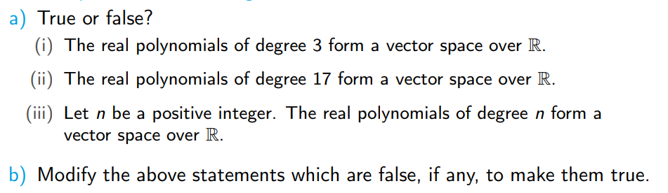
Example 3 (The set of polynomials of degree 3)
This seems like a 180, however, looking closely, the set consists of polynomials only of degree 3. Unlike the definition of $\mathbb{P}_n(\mathbb{F})$ which allows any polynomial with degree $\leq n$, the degree must be precisely $n$ in this case. This violates Axiom 1 as:

$$\begin{align*} \text{let } p(x) = x^3 + 2x, \\ \text{let } q(x) = -x^3+5, \\ p(x)+q(x)=2x+5 \end{align*}$$

Since both $p$ and $q$ are within the set, performing an addition between the two results in a polynomial outside of the set, hence not being closed. We can generalise this to be true for any $n$.

Answering these,

• a)
  • (i) False, see Example 3
  • (ii) False, see Example 3
  • (iii) False, see Example 3
• b)
  Simply restate it to be less than or equal to each degree in order to be true

6.2 Vector Arithmetic#

The axioms give a minimal set of rules needed to define a vector space. The first five vector space axioms apply to vector addition, and they are in fact identical to the five basic axioms of addition for integers, real numbers and complex numbers. This means that all the arithmetic properties of vector addition are identical to corresponding properties of addition of numbers.

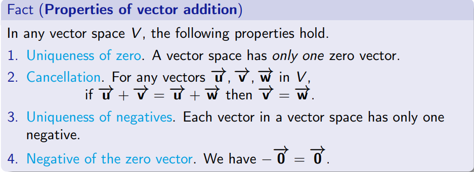
Proposition 1. In any vector space $V$, the following properties hold for addition.

1. Uniqueness of Zero. There is one and only one zero vector.
2. Cancellation Property. If $\mathbf{u}, \mathbf{v}, \mathbf{w} \in V$ satisfy $\mathbf{u} + \mathbf{v} = \mathbf{u} + \mathbf{w}$, then $\mathbf{v} = \mathbf{w}$.
3. Uniqueness of Negatives. For all $\mathbf{v} \in V$, there exists only one $\mathbf{w} \in V$ such that $\mathbf{v} + \mathbf{w} = 0$

Proof

Prove (3): Each vector in a vector space only has one negative.
Let $\mathbf{v} + \mathbf{w} = \mathbf{0}$ and $\mathbf{v} + \mathbf{u} = \mathbf{0}$. By the axioms of a vector space, we can evaluate $\mathbf{w}$ as follows:

$$\begin{align*} \mathbf{w} &= \mathbf{w} + \mathbf{0} \\ \mathbf{w} &= \mathbf{w} + (\mathbf{v} + \mathbf{u}) \\ \mathbf{w} &= (\mathbf{w} + \mathbf{v}) + \mathbf{u} \\ \mathbf{w} &= \mathbf{0} + \mathbf{u} \\ \mathbf{w} &= \mathbf{u} \quad \quad \quad \quad \quad \quad \quad \quad \quad \blacksquare. \end{align*}$$

Prove (4): The zero vector is its own negative i.e. $\mathbf{0}=\mathbf{-0}$
By the existence of the zero vector, we know that adding $\mathbf{0}$ to itself yields:

$$\begin{align*} \mathbf{0} + \mathbf{0} &= \mathbf{0} \end{align*}$$

By the definition of an additive inverse, the negative of the zero vector, $-\mathbf{0}$, must satisfy:

$$\begin{align*} \mathbf{0} + (-\mathbf{0}) &= \mathbf{0} \end{align*}$$

Since both expressions equal $\mathbf{0}$, we can equate them:

$$\begin{align*} \mathbf{0} + \mathbf{0} &= \mathbf{0} + (-\mathbf{0}) \end{align*}$$

Because the additive inverse is unique, it must follow that:

$$\begin{align*} \mathbf{0} &= -\mathbf{0} \quad \quad \quad \quad \blacksquare. \end{align*}$$

Proposition 2. Suppose that $V$ is a vector space over a field $\mathbb{F}$, $\lambda \in \mathbb{F}$, $\mathbf{v} \in \mathbb{F},0$ is the zero scalar in $\mathbb{F}$ and $\mathbf{0}$ is the zero vector in $V$. Then the following properties hold for multiplication by a scalar:

1. Multiplication by the zero scalar. $\mathbf{0} \mathbf{v} = \mathbf{0}$,
2. Multiplication of the zero vector. $\lambda \mathbf{0}=\mathbf{0}.$
3. Multiplication by $-1$. $(-1)\mathbf{v}=-\mathbf{v}$ (the additive inverse of $\mathbf{v}$).
4. Zero Products. If $\lambda \mathbf{v} = \mathbf{0}$, then either $\lambda = 0$ or $\mathbf{v} = \mathbf{0}$.
5. Cancellation Property. If $\lambda \mathbf{v} = \mu \mathbf{v}$ and $\mathbf{v} \neq \mathbf{0}$ then $\lambda = \mu$.

6.3 Subspaces#

Many problems about vectors involve subsets of some vector space, such as the points on a line in $\mathbb{R}^n$ forming a subset of $\mathbb{R}^n$, or the points on a plane in $\mathbb{R}^3$ form a subset of $\mathbb{R}^n$.

The question that arises is if a subset of the real-number line is a vector space; for now we will focus on ways to show that a given set is not a vector space.

Example. Suppose you have $S = [-5,5] = \{x \in \mathbb{R}: -5 \leq x \leq 5 \}$, is this a vector space?
Geometrically, the set S represents a line segment.

The given system is not a vector space, since it is not closed under scalar multiplication. A counterexample; $5 \in S$, but 5 + 5 = 10 is not an element of S.

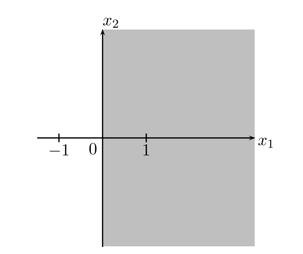
Example. The plane $\mathbb{R}^2$ is a vector space. Show that the subset $S$ of $\mathbb{R}^2$ given by

$$S = \left\{ \mathbf{x}= \pmatrix{x_1 \\ x_2} \in \mathbb{R^2}: x_1 \geq 0 \right\}$$

is not a vector space.

There are several ways to solve this problem since there are several axioms which are not satisfied. One method is to note that $\pmatrix{1 \\ 0} \in S$, whereas $-1\pmatrix{1 \\ 0} = \pmatrix{-1 \\ 0} \notin S$. Hence the set $S$ is not closed under scalar multiplication and so $S$ is not a vector space.

Geometric view of S

Example. Let $S = {p\in \mathbb{P(R)} : p(2) \geq 0}$. Is $S$ a vector space?

Suppose $p(x)=x^2$, then $p \in S$ as $p(2)=4 \ge 0$, but $-p$ is not in $S$ as $-p(2)=-4$, therefore $S$ is not a vector space.

• A common theme here is in showing that a set does not need to contain some region (i.e. negatives), you should always give a specific numerical example. You should do the same when showing that a set is not closed under addition, or not closed under scalar multiplication.

However, you can (sometimes) use these methods to show that something is not a vector space, but you can never use them to show that something is a vector space; (basically some vs all proof in 1081).

So far we have seen that it is usually fairly simple to show that a subset is not a vector space, but it will be time-consuming and tedious to show that a given subset is a vector space by checking all ten axioms. We can leverage the fact that they are subsets to make things simpler.

We first make the following definitions,

A simple test for a subspace is given by the following theorem.

Proof. If $S$ is a subspace then it is a vector space.

Suppose $S$ contains the zero vector and the two closure axioms 1 and 6 are satisfied by elements of $S$. Since $V$ is a vector space, and $S$ and $V$ are under the same operations, the vector space axioms 2, 3, 7, 8, 9, 10 are automatically satisfied by all elements of S.

Since $S$ contains the zero vector, if $\mathbf{v} \in S$, then $\mathbf{0+v=0}$ (since this is true in $V$ and hence in $S$, so axiom 4 follows).

Finally, if $v\in S$ then $v\in V$ . Hence, from part 3 of Proposition 2, we have $−\mathbf{v} = (−1)\mathbf{v}$. But, as $S$ is closed under multiplication by a scalar, we have $(−1)\mathbf{v} ∈ S$, and hence $−\mathbf{v} ∈ S$. Thus, axiom 5 is satisfied for all vectors in S. The proof is complete.

If we want to check if $S$ is a subspace of $V$, we should first check if the zero vector of $V$ is in $S$. If the zero vector is in $S$ we can proceed to verify the two closure axioms. Otherwise, we can draw a conclusion that $S$ is not a subspace of $V$. If we have proved that axioms 1, 4 and 6 are true, then axiom 5 also works automatically and need not be checked separately.

Identifying the Subspace#

In order to use the subset theorem, you will need to identify a vector space containing your set $S$.
This is where to look: In all the sets below, $m$ and $n$ are positive integers and $\mathbb{F}$ is a field. Usually, $\mathbb{F}$ is $\mathbb{Q}$, $\mathbb{R}$or $\mathbb{C}$. Recall:

• $\mathbb{R}^n$ is a vector space over the field $\mathbb{R}$.
• $\mathbb{C}^n$ is a vector space over the field $\mathbb{C}$ (and also over the field $\mathbb{R}$).
• $\mathbb{P}(\mathbb{F})$, the set of polynomials with coefficients in the field $\mathbb{F}$, is a vector space over $\mathbb{F}$.
• $\mathbb{P}_n(\mathbb{F})$, the set of polynomials of degree at most $n$ with coefficients in the field $\mathbb{F}$, is a vector space over $\mathbb{F}$.
• $M_{mn}(\mathbb{F})$, the set of matrices with $m$ rows and $n$ columns and with entries in the field $\mathbb{F}$, is a vector space over $\mathbb{F}$.

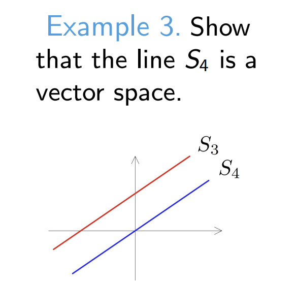
Example.

Proof. Since $S_4$ is a subset of the known vector space $\mathbb{R}^2$, we only need to verify the three conditions of the Subspace Theorem to prove it is a vector space.

1. The zero vector is in $S_4$:
Let $\vec{\mathbf{x}} = \begin{pmatrix} 0 \\ 0 \end{pmatrix}$. We test if it satisfies the rule of the set by substituting $x_1 = 0$ and $x_2 = 0$:

$$2(0) - 3(0) = 0$$

Since the condition is satisfied, the zero vector $\vec{\mathbf{0}} \in S_4$.

2. Closure under addition:
Let $\vec{\mathbf{u}}$ and $\vec{\mathbf{v}}$ be two random vectors in $S_4$. By definition of the set, this means we know as a fact that $2u_1 - 3u_2 = 0$ and $2v_1 - 3v_2 = 0$.
We want to test if their sum, $\vec{\mathbf{u}} + \vec{\mathbf{v}} = \begin{pmatrix} u_1 + v_1 \\ u_2 + v_2 \end{pmatrix}$, also satisfies the rule of the set.

$$\begin{align*} 2(u_1 + v_1) - 3(u_2 + v_2) &= 2u_1 + 2v_1 - 3u_2 - 3v_2 \\ &= (2u_1 - 3u_2) + (2v_1 - 3v_2) \\ &= 0 + 0 \\ &= 0 \end{align*}$$

Because the result is $0$, the sum vector survives the test, meaning $\vec{\mathbf{u}} + \vec{\mathbf{v}} \in S_4$.

3. Closure under scalar multiplication:
Let $\vec{\mathbf{u}} \in S_4$ (so $2u_1 - 3u_2 = 0$) and let $\lambda$ be any real scalar.
We want to test if the scaled vector, $\lambda\vec{\mathbf{u}} = \begin{pmatrix} \lambda u_1 \\ \lambda u_2 \end{pmatrix}$, satisfies the rule.

$$\begin{align*} 2(\lambda u_1) - 3(\lambda u_2) &= \lambda(2u_1) - \lambda(3u_2) \\ &= \lambda(2u_1 - 3u_2) \\ &= \lambda(0) \\ &= 0 \end{align*}$$

Because the result is $0$, the scaled vector survives the test, meaning $\lambda\vec{\mathbf{u}} \in S_4$.

Because $S_4$ contains the zero vector and is closed under both addition and scalar multiplication, it is a valid subspace of $\mathbb{R}^2$, and therefore it is a vector space itself.
$\blacksquare$.

Example. Show that $S = \left\{\mathbf{x} \in \mathbb{R}^2:2x_1-3x_2=0\right\}$ is a vector space.
Proof. We can rewrite the equation $2x_1-3x_2=0$ as $x_2=\dfrac{2}{3}x_1$, and then let $S$ be the subset of $\mathbb{R}^2$ defined by vectors of the form $\begin{pmatrix} x \\ \frac{2}{3}x \end{pmatrix}$ where $x \in \mathbb{R}$. We can then verify the three subspace conditions.

1. The zero vector is in $S$:
If we choose $x = 0$, the resulting vector in our set is:

$$\begin{pmatrix} 0 \\ \frac{2}{3}(0) \end{pmatrix} = \begin{pmatrix} 0 \\ 0 \end{pmatrix}$$

Since we can generate the zero vector, $\vec{\mathbf{0}} \in S$.

2. Closure under addition:
Let $\vec{\mathbf{u}}$ and $\vec{\mathbf{v}}$ be two vectors in $S$. By definition of the set, they must have the form:

$$\vec{\mathbf{u}} = \begin{pmatrix} a \\ \frac{2}{3}a \end{pmatrix} \quad \text{and} \quad \vec{\mathbf{v}} = \begin{pmatrix} b \\ \frac{2}{3}b \end{pmatrix}$$

We add them together:

$$\begin{align*} \vec{\mathbf{u}} + \vec{\mathbf{v}} &= \begin{pmatrix} a \\ \frac{2}{3}a \end{pmatrix} + \begin{pmatrix} b \\ \frac{2}{3}b \end{pmatrix} \\ &= \begin{pmatrix} a + b \\ \frac{2}{3}a + \frac{2}{3}b \end{pmatrix} \\ &= \begin{pmatrix} a + b \\ \frac{2}{3}(a + b) \end{pmatrix} \end{align*}$$

Notice that the bottom component is exactly $\frac{2}{3}$ times the top component. Because the sum perfectly matches the required pattern of the set, $\vec{\mathbf{u}} + \vec{\mathbf{v}} \in S$.

3. Closure under scalar multiplication:
Let $\vec{\mathbf{u}} = \begin{pmatrix} a \\ \frac{2}{3}a \end{pmatrix}$ be in $S$, and let $\lambda$ be any real scalar.
We scale the vector:

$$\begin{align*} \lambda\vec{\mathbf{u}} &= \lambda \begin{pmatrix} a \\ \frac{2}{3}a \end{pmatrix} \\ &= \begin{pmatrix} \lambda a \\ \lambda\left(\frac{2}{3}a\right) \end{pmatrix} \\ &= \begin{pmatrix} \lambda a \\ \frac{2}{3}(\lambda a) \end{pmatrix} \end{align*}$$

Once again, the bottom component is exactly $\frac{2}{3}$ times the top component. The scaled vector maintains the pattern, so $\lambda\vec{\mathbf{u}} \in S$.

Since $S$ contains the zero vector and is closed under addition and scalar multiplication, it is a subspace of $\mathbb{R}^2$.

You can do it both ways; you can rewrite a given equation into a vector form or you can simply just use the equation as in previous examples.

Lemma. A line in $\mathbb{R}^n$ is a subspace if and only if it passes through the origin;
Suppose that $S$ represents a line in $\mathbb{R}^n$. If $\mathbf{0} \notin S$, then $S$ is not a subspace. Hence, a line which does not pass through the origin is not a vector subspace.
If $S$ is a line through the origin we can write

$$S = \left\{ \mathbf{x} \in \mathbb{R}^n : \mathbf{x}=t\mathbf{v}, t \in \mathbb{R}\right\},$$

where $\mathbf{v}$ is a fixed non-zero vector in $\mathbb{R}^n$. To check if $S$ is a subspace we check the two closure axioms.
Closure under addition. If $\mathbf{x}_1, \mathbf{x}_2 \in S$ then

$$\mathbf{x}_1 = t_1\mathbf{v} \quad \text{and} \quad \mathbf{x}_2 = t_2\mathbf{v} \quad \text{for some } t_1, t_2 \in \mathbb{R}.$$

Hence,

$$\mathbf{x}_1 + \mathbf{x}_2 = (t_1 + t_2)\mathbf{v} = t'\mathbf{v},$$

where $t' = t_1 + t_2 \in \mathbb{R}$. Thus, $\mathbf{x}_1 + \mathbf{x}_2 \in S$, and hence $S$ is closed under addition.
Closure under multiplication by a scalar. We have

$$\mathbf{x} = t\mathbf{v} \quad \text{for some} \quad t \in \mathbb{R},$$

and hence, if $\lambda \in \mathbb{R}$,

$$\lambda\mathbf{x} = \lambda(t\mathbf{v}) = (\lambda t)\mathbf{v} = t''\mathbf{v},$$

where $t'' = \lambda t \in \mathbb{R}$. Hence $\lambda\mathbf{x} \in S$, and thus $S$ is closed under multiplication by a scalar.
Therefore, by the Subspace Theorem, the line $S$ is a subspace of $\mathbb{R}^n$ if it passes through the origin. A similar result to that given for lines also holds for planes.

Example. Let $S$ be the set of polynomials which satisfy all of the following conditions:

• their coefficients are complex numbers,
• their degree is at most 7,
• their second derivative evaluated at $x=5$ is zero.
  Is $S$ a vector space over $\mathbb{C}$?

Rewriting $S$ in set notation,

$$S=\left\{ p \in \mathbb{P}_7(\mathbb{C}) : p''(5)=0 \right\}.$$

By the Subspace Theorem, we only check axioms 1, 4 and 6;
Closure of vector addition:
Suppose $p,q \in S$, then $p''(5) = 0, q''(5)=0$, if we let $h = p + q$, then

$$\begin{align*} h''(5)&=p''(5)+q''(5) \\ h''(5) &= 0 + 0 \\ h''(5) &= 0 \end{align*}$$

meaning that vector addition is closed.

Closure under scalar multiplication:
Suppose $p\in S$, then $p''(5) = 0$, suppose $c$ is some constant in $\mathbb{C}$, and $h(x)=c \cdot p(x)$, so

$$\begin{align*} h''(x)&= c \cdot p''(x) \\ h''(5)&=c \cdot p''(5) \\ h''(5) &= c \cdot 0 \\ h''(5) &= 0. \end{align*}$$

Therefore, scalar multiplication is also closed (and hence negatives of vectors).

Existence of a 0 vector:
If $p\in S$, $p''(5) = 0$, but if $p(x) = 0$ then $p''(5)$ is also equal to zero.

In practice, some of the most important subspaces of $\mathbb{R}^n$ are connected with systems of linear equations, that is, with the matrix equation $A\mathbf{x}=\mathbf{b}$.
Example. Let $A$ be an $m × n$ matrix with real entries. Show that the subset $S$ of $\mathbb{R}^n$ which consists of all solutions of the matrix equation $A\mathbf{x}=\mathbf{b}$ for given $\mathbf{b} \in \mathbb{R}^m$ is a subspace of $\mathbb{R}^n$ if and only if $\mathbf{b} = \mathbf{0}$.

Suppose there exists a case where $\mathbf{b} \neq \mathbf{0}$, then $\mathbf{0} \in \mathbb{R}^n$ is not a solution of $A\mathbf{x}=\mathbf{b}$ as $A\mathbf{0}=\mathbf{0} \neq\mathbf{b}$, and hence $S$ does not contain the zero vector. Thus $S$ is not a subspace.

If $\mathbf{b} = \mathbf{0}$, then $S$ is the set of solutions of $A\mathbf{x}=\mathbf{0}$. We use the Subspace Theorem to show that $S$ is a subspace.
Closure under addition. If $\mathbf{x} \in S$ and $\mathbf{y} \in S$, then $A\mathbf{x}=\mathbf{0}$ and $A\mathbf{y}=\mathbf{0}$, and hence

$$A\mathbf{(x+y)}=A\mathbf{x}+A\mathbf{y}=\mathbf{0}+\mathbf{0}=\mathbf{0}$$

Thus $\mathbf{x}+\mathbf{y}\in S$ and $S$ is closed under addition.
Closure under multiplication by a scalar. If $\mathbf{x} \in S$, we have $A \mathbf{x}= \mathbf{0},$ and hence for all $\lambda \in \mathbb{R}$,

$$A(\lambda \mathbf{x}) = \lambda A( \mathbf{x}) = \lambda \mathbf{0} = \mathbf{0}.$$

And hence is it closed under scalar multiplication.

Example. (Rapid-fire subspace drills) For each of the following sets, decide whether $S$ is a subspace. Each one hides a different trap.

(a) $S = \left\{ \mathbf{x} \in \mathbb{R}^3 : x_1 + x_2 + x_3 = 1 \right\}$.
Not a subspace. Substituting the zero vector gives $0 + 0 + 0 = 0 \neq 1$, so $\mathbf{0} \notin S$ and we can stop immediately. Always test the zero vector first; if it fails you are done in one line.

(b) $S = \left\{ \mathbf{x} \in \mathbb{R}^2 : x_1 x_2 = 0 \right\}$, i.e. the union of the two coordinate axes.
Not a subspace. It contains $\mathbf{0}$, and it is even closed under scalar multiplication since $(\lambda x_1)(\lambda x_2) = \lambda^2 x_1x_2 = 0$; however it is not closed under addition:

$$\begin{pmatrix} 1 \\ 0 \end{pmatrix} + \begin{pmatrix} 0 \\ 1 \end{pmatrix} = \begin{pmatrix} 1 \\ 1 \end{pmatrix} \notin S.$$

Passing two of the three conditions means nothing; all three must hold.

(c) $S = \left\{ \mathbf{x} \in \mathbb{R}^3 : x_1 = x_2 = x_3 \right\}$.
Subspace. Every element has the form $t\begin{pmatrix} 1 \\ 1 \\ 1\end{pmatrix}$ for $t \in \mathbb{R}$, so $S$ is a line through the origin, and we proved in the Lemma above that such lines are subspaces.

(d) $S = \left\{ A \in M_{22}(\mathbb{R}) : \det(A) = 0 \right\}$.
Not a subspace. The zero matrix is in $S$, and $\det(\lambda A) = \lambda^2\det(A) = 0$ gives closure under scalar multiplication, but addition fails:

$$\begin{pmatrix} 1 & 0 \\ 0 & 0 \end{pmatrix} + \begin{pmatrix} 0 & 0 \\ 0 & 1 \end{pmatrix} = \begin{pmatrix} 1 & 0 \\ 0 & 1 \end{pmatrix},$$

and the identity matrix has determinant $1 \neq 0$, so the sum has escaped the set.

The lesson from these drills: sets defined by linear, homogeneous conditions (like $2x_1 - 3x_2 = 0$ or $p''(5) = 0$) tend to be subspaces, while sets defined by non-linear conditions (products, determinants, inequalities) or by conditions with a non-zero right hand side tend to fail.

An important theoretical and practical problem concerning vector spaces is that of finding all their subspaces. For example, it can be shown that the only subspaces of $\mathbb{R}^2$ are (1) the origin, (2) lines through the origin, and (3) $\mathbb{R}^2$ itself. Similarly, for $\mathbb{R}^3$ the only subspaces are (1) the origin, (2) lines through the origin, (3) planes through the origin, and (4) $\mathbb{R}^3$ itself. A listing of subspaces can be given for any vector space. However, before we can investigate this problem satisfactorily, we require further machinery. This machinery will be developed in Sections 6.4 and 6.5. In vector spaces other than $\mathbb{R}^n$ it may be difficult to get a good geometric feel for which subsets are subspaces. Nonetheless, the Subspace Theorem allows one a simple way to check whether a certain set is a subspace or not.

6.4 Linear combinations and spans#

The two fundamental vector space operations are addition and multiplication by a scalar. If we combine these two we can result in something called "linear combinations" and "span"; a linear combination of a given set of vectors is a sum of scalar multiples of the vectors and the span of a given set of vectors is the set of all linear combinations of the vectors.

$$\lambda_1 \mathbf{v_1}+ \cdots + \lambda_n \mathbf{v_n} \text{ with } \lambda_1, \cdots, \lambda_n \in \mathbb{F}. >$$

Example. The vector $\begin{pmatrix}3 \\ -4 \end{pmatrix}$ is a linear combination of the vectors in the set

$$\left \{ \begin{pmatrix} 1 \\ 1 \end{pmatrix} , \begin{pmatrix} 2 \\ 3 \end{pmatrix} , \begin{pmatrix} 1 \\ -1 \end{pmatrix} \right \} \text { in } \mathbb{R}^2 \text{ because } \begin{pmatrix} 3 \\ -4 \end{pmatrix} = 2\begin{pmatrix} 1 \\ 1 \end{pmatrix} + (-1)\begin{pmatrix} 2 \\ 3 \end{pmatrix} + 3\begin{pmatrix} 1 \\ -1 \end{pmatrix} .$$

Example. Is $\mathbf{b} = \begin{pmatrix} 3 \\ -1 \\ 5 \end{pmatrix}$ a linear combination of $\mathbf{v}_1 = \begin{pmatrix} 1 \\ 1 \\ 1 \end{pmatrix}$ and $\mathbf{v}_2 = \begin{pmatrix} 1 \\ -1 \\ 2 \end{pmatrix}$?

We are looking for scalars $\lambda_1, \lambda_2$ such that $\lambda_1\mathbf{v}_1 + \lambda_2\mathbf{v}_2 = \mathbf{b}$. Comparing components gives three equations in only two unknowns:

$$\begin{align*} \lambda_1 + \lambda_2 &= 3, \\ \lambda_1 - \lambda_2 &= -1, \\ \lambda_1 + 2\lambda_2 &= 5. \end{align*}$$

Adding the first two equations,

$$\begin{align*} 2\lambda_1 &= 2 \\ \lambda_1 &= 1, \end{align*}$$

and hence $\lambda_2 = 3 - 1 = 2$. Substituting into the third equation as a check: $1 + 2(2) = 5$, which is consistent. Therefore

$$\mathbf{b} = \mathbf{v}_1 + 2\mathbf{v}_2,$$

so $\mathbf{b}$ is a linear combination of the two vectors. Notice that if the third component of $\mathbf{b}$ were changed to, say, $4$, the first two equations would still force $\lambda_1 = 1$ and $\lambda_2 = 2$, but then $\lambda_1 + 2\lambda_2 = 5 \neq 4$ and no combination would exist. This makes sense geometrically; in $\mathbb{R}^3$ the set of all linear combinations of two (non-parallel) vectors is only a plane, so most vectors miss it.

We know that a vector space is closed under addition and multiplication of scalars, and therefore any subspace of that vector space is closed as well, so it must be closed under the operation of forming linear combinations.

Example. The span of a non-zero vector $\mathbf{v}$ in $\mathbb{R}^n$ is a line through the origin;

$$S = \left \{\mathbf{x} \in \mathbb{R}^n: \mathbf{x}= \lambda \mathbf{v}, \text{ for some } \lambda \in \mathbb{R} \right \}.$$

This set is just span($\mathbf{v}$).

Example. If $\left \{ \mathbf{v}, \mathbf{w} \right \}$ is a pair of non-zero, non-parallel vectors in $\mathbb{R}^n$ then span($\mathbf{v}, \mathbf{w}$) is a plane containing the origin.

Proof. We first note that $\mathbf{0} \in S$, since we may take each scalar to be zero. We know that every linear combination of $S$ is a vector in $V$, so $\text{span}(S)$ is a subset of $V$.

To prove that $\text{span}(S)$ is a subspace we will use the Subspace Theorem, so we set out to prove that $\text{span}(S)$ is closed under addition and under multiplication by scalars. Let $S$ be the set

$$S = \{\mathbf{v}_1, \dots, \mathbf{v}_n\}$$

where all $\mathbf{v}_j$ belong to $V$.
To show closure under addition, suppose $\mathbf{u}, \mathbf{w} \in \text{span}(S)$. Then

$$\begin{aligned} \mathbf{u} &= \lambda_1 \mathbf{v}_1 + \cdots + \lambda_n \mathbf{v}_n \quad \text{for some } \lambda_1, \dots, \lambda_n \in \mathbb{F} \quad \text{and} \\ \mathbf{w} &= \mu_1 \mathbf{v}_1 + \cdots + \mu_n \mathbf{v}_n \quad \text{for some } \mu_1, \dots, \mu_n \in \mathbb{F}, \\ \text{so} \quad \mathbf{u} + \mathbf{w} &= (\lambda_1 + \mu_1)\mathbf{v}_1 + \cdots + (\lambda_n + \mu_n)\mathbf{v}_n \quad \text{with } \lambda_1 + \mu_1, \dots, \lambda_n + \mu_n \in \mathbb{F}. \end{aligned}$$

This shows that $\mathbf{u} + \mathbf{w}$ belongs to $\text{span}(S)$, so $\text{span}(S)$ is closed under addition. To prove closure under multiplication by a scalar, suppose $\mathbf{u} \in \text{span}(S)$ and $\lambda \in \mathbb{F}$. Then

$$\begin{aligned} \lambda \mathbf{u} &= \lambda(\lambda_1 \mathbf{v}_1 + \cdots + \lambda_n \mathbf{v}_n) \\ &= (\lambda \lambda_1)\mathbf{v}_1 + \cdots + (\lambda \lambda_n)\mathbf{v}_n, \end{aligned}$$

where $\lambda \lambda_1, \dots, \lambda \lambda_n \in \mathbb{F}$. This shows that $\lambda \mathbf{u}$ belongs to $\text{span}(S)$, so $\text{span}(S)$ is closed under multiplication by scalars.

We have now proved that $\text{span}(S)$ is a subspace of $V$. To show that it is the smallest subspace of $V$ containing $S$, suppose $W$ is any subspace of $V$ containing $S$. Then $W$ is itself a vector space containing $S$ and, by what we have just proved, $\text{span}(S)$ is a subspace of $W$. This completes the proof by showing that $\text{span}(S)$ is a subspace of every subspace of $V$ containing $S$.

Example. Every vector $\begin{pmatrix} x_1 \\ \vdots \\ x_n \end{pmatrix} \in \mathbb{R}^n$ can be written as $\mathbf{x}=x_1\mathbf{e}_1 + \cdots + x_n \mathbf{e}_n$. This expresses $\mathbf{x}$ as a linear combination of the set $\{\mathbf{e}_1,\cdots,\mathbf{e}_n\}$, where

$$\mathbf{e}_1=\begin{pmatrix} 1 \\ 0 \\ \vdots \\ 0 \end{pmatrix}, \mathbf{e}_2=\begin{pmatrix} 0 \\ 1 \\ \vdots \\ 0 \end{pmatrix}, \cdots, \mathbf{e}_n=\begin{pmatrix} 0 \\ 0 \\ \vdots \\ 1 \end{pmatrix}.$$

Thus, $\mathbb{R}^n =$ span$(\mathbf{e}_1,\cdots,\mathbf{e}_n)$ and the set $\{\mathbf{e}_1,\cdots,\mathbf{e}_n\}$ spans $\mathbb{R}^n$.

Example. Let $\mathbb{P}_n$ denote the space of polynomials of degree less than or equal to $n$. Every polynomial $p \in \mathbb{P}_n$ can be written as a linear combination of the polynomials $\{1, x, x_2 , \cdots, x_n\}$, so $\mathbb{P}_n = \text{span}(1, x, x_2 , \cdots, x_n)$ . We shall see later that there is no finite set of vectors whose span is all of $\mathbb{P}$ (the vector space of all polynomials).

6.4.1 Matrices and spans in $\mathbb{R}^m$#

We want to have an effective way to tell whether or not a given vector in $\mathbb{R}^m$ belongs to the span of a set $S = \{\mathbf{v}_1, \dots, \mathbf{v}_n\}$. From the definition of span, we know that $\mathbf{b}$ belongs to $\text{span}(S)$ if and only if there are $\lambda_1, \dots, \lambda_n \in \mathbb{R}$ such that

$$\mathbf{b} = \lambda_1\mathbf{v}_1 + \cdots + \lambda_n\mathbf{v}_n.$$

This equivalent to the condition that there is at least one solution to the vector equation

$$x_1\mathbf{v}_1 + \cdots + x_n\mathbf{v}_n = \mathbf{b},$$

where $x_1, \dots, x_n$ are the unknowns. This vector equation represents a set of simultaneous linear equations in $n$ unknowns. Therefore the question of whether $\mathbf{b}$ belongs to $\text{span}(S)$ is a question of whether or not a particular set of linear equations has a solution. This is the sort of question which we studied in detail in MATH1131/41.

Furthermore, suppose that $\mathbf{v}_1 = \begin{pmatrix} a_{11} \\ \vdots \\ a_{m1} \end{pmatrix}$, $\mathbf{v}_2 = \begin{pmatrix} a_{12} \\ \vdots \\ a_{m2} \end{pmatrix}$, $\dots$, $\mathbf{v}_n = \begin{pmatrix} a_{1n} \\ \vdots \\ a_{mn} \end{pmatrix}$, and $\mathbf{x} = \begin{pmatrix} x_1 \\ \vdots \\ x_n \end{pmatrix}$.

If that $A$ is the $m \times n$ matrix whose columns are the vectors $\mathbf{v}_1, \dots, \mathbf{v}_n$ then

$$\begin{aligned} A\mathbf{x} &= \begin{pmatrix} a_{11} & \cdots & a_{1n} \\ \vdots & \ddots & \vdots \\ a_{m1} & \cdots & a_{mn} \end{pmatrix} \begin{pmatrix} x_1 \\ \vdots \\ x_n \end{pmatrix} = \begin{pmatrix} a_{11}x_1 + \cdots + a_{1n}x_n \\ \vdots \\ a_{m1}x_1 + \cdots + a_{mn}x_n \end{pmatrix} \\ &= x_1 \begin{pmatrix} a_{11} \\ \vdots \\ a_{m1} \end{pmatrix} + \cdots + x_n \begin{pmatrix} a_{1n} \\ \vdots \\ a_{mn} \end{pmatrix} = x_1\mathbf{v}_1 + \cdots + x_n\mathbf{v}_n. \end{aligned}$$

As a result, we have the following proposition.

Proposition 3 (Matrices, Linear Combinations and Spans). If $S = \{\mathbf{v}_1, \dots, \mathbf{v}_n\}$ is a set of vectors in $\mathbb{R}^m$ and $A$ is the $m \times n$ matrix whose columns are the vectors $\mathbf{v}_1, \dots, \mathbf{v}_n$ then

a) a vector $\mathbf{b}$ in $\mathbb{R}^m$ can be expressed as a linear combination of $S$ if and only if it can be expressed in the form $A\mathbf{x}$ for some $\mathbf{x}$ in $\mathbb{R}^n$,

b) a vector $\mathbf{b}$ in $\mathbb{R}^m$ belongs to $\text{span}(S)$ if and only if the equation $A\mathbf{x} = \mathbf{b}$ has a solution $\mathbf{x}$ in $\mathbb{R}^n$.

Example 10. For the set of three vectors

$$\mathbf{v}_1 = \begin{pmatrix} 0 \\ 5 \\ 3 \\ 6 \end{pmatrix}, \mathbf{v}_2 = \begin{pmatrix} 1 \\ 3 \\ 4 \\ 5 \end{pmatrix}, \mathbf{v}_3 = \begin{pmatrix} -2 \\ -3 \\ -5 \\ -6 \end{pmatrix} \in \mathbb{R}^4, \quad \text{we let} \quad A = \begin{pmatrix} 0 & 1 & -2 \\ 5 & 3 & -3 \\ 3 & 4 & -5 \\ 6 & 5 & -6 \end{pmatrix} \quad \text{and} \quad \mathbf{x} = \begin{pmatrix} x_1 \\ x_2 \\ x_3 \end{pmatrix}.$$