The graph of a function f of one variable, given by y=f(x), gives rise to a curve in R2. The graph of a function F of two variables, given by z=F(x,y), gives rise to a surface in R3.
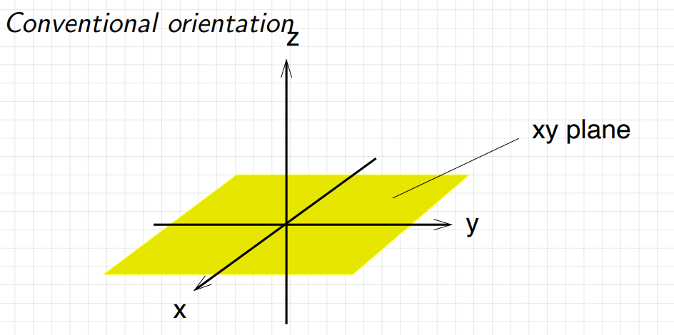
Sketching a graph in R3 can be challenging because the sketch must be represented in R2. The conventional orientation is as follows:
This is however difficult to properly represent for plots that cannot be visualised clearly from a fixed perspective, and also cannot be easily drawn by hand.
Topographic maps solve this problem by using contour lines to represent the height (above sea level) of the surface of the earth at various points. This idea can be adapted to sketching a surface z=F(x,y) described by a function F. Here, z represents the height of the surface above the xy-plane, and the contours of the surface can be defined as follows:
Note
Contour
A contour or level curve of a function F:R2→R is a curve in R2 corresponding to an equation of the form F(x,y)=C, where C is a constant.
For each level curve, the corresponding value of C gives the height of the curve above the xy-plane.
We can use a profile obtained from a plot of:
z versus y (with x=constant) or
z versus x (with y=constant).
These can be thought of as vertical cuts through the function surface.
Basically level curves are top-down view; profile's are views from the side of the plane when seen in conventional orientation.
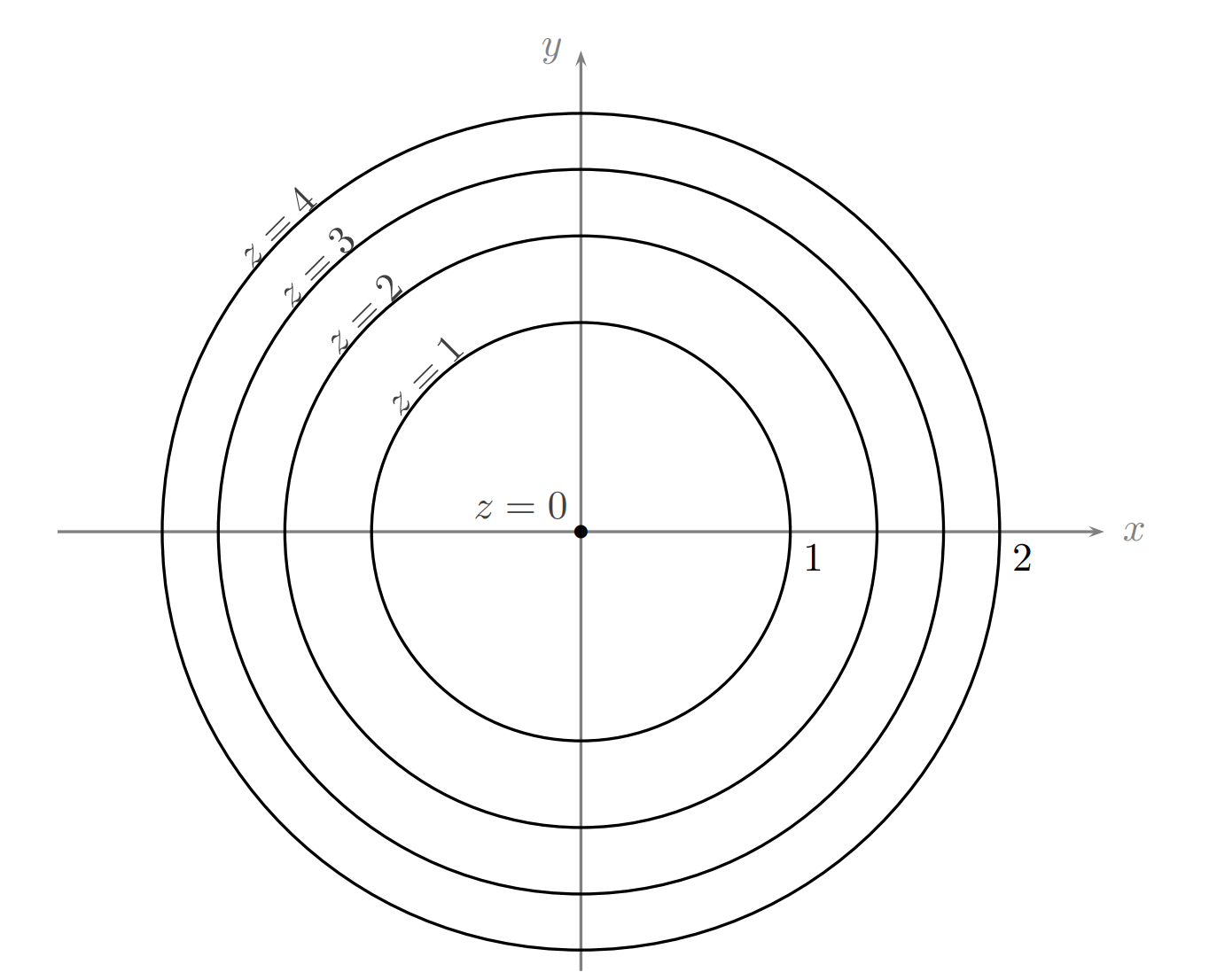
Example Sketch level curves for the function F:R2→R, where F(x,y)=x2+y2.
Since the level curves are of the form x2+y2=C, where C is nonnegative (as there is no solution for C<0), you can interpret this as circles with varying radii.
These are the level curves given by x2+y2={0,1,2,3,4}.
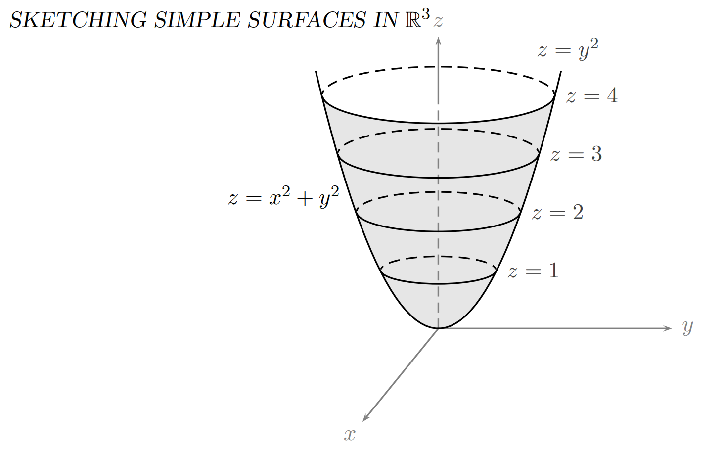
Example Sketch the surface in R3 described by the equation z=x2+y2.
From the previous example, we know that the surface increases in radius on the xy-plane; the level curves for the surface are circles. When x=0, we have z=y2. On the yz-plane, this is simply a parabola. The yz-profile and level curves help produce a sketch of the surface.
(You can also use the xz-profile but since they are both the same you can just use one)
This is the conventional orientation for the x-, y- and z-axes.
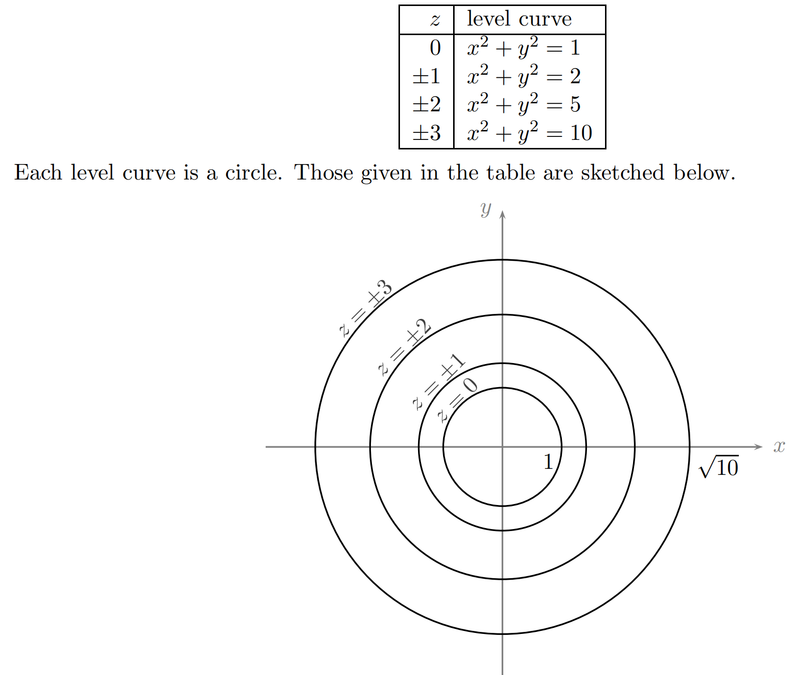
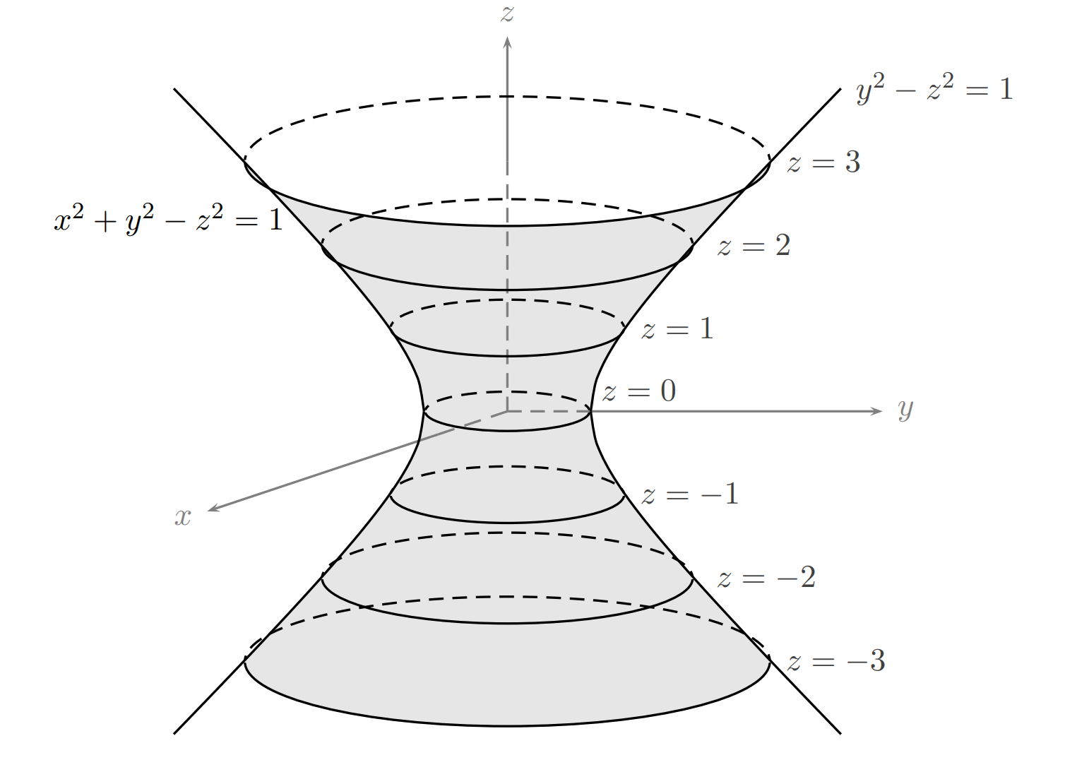
Example A surface in R3 is described by the equation x2+y2−z2=1. Sketch some level curves and hence sketch the surface in R3 .
First obtain the level curve by setting z equal to C, for some constant C.
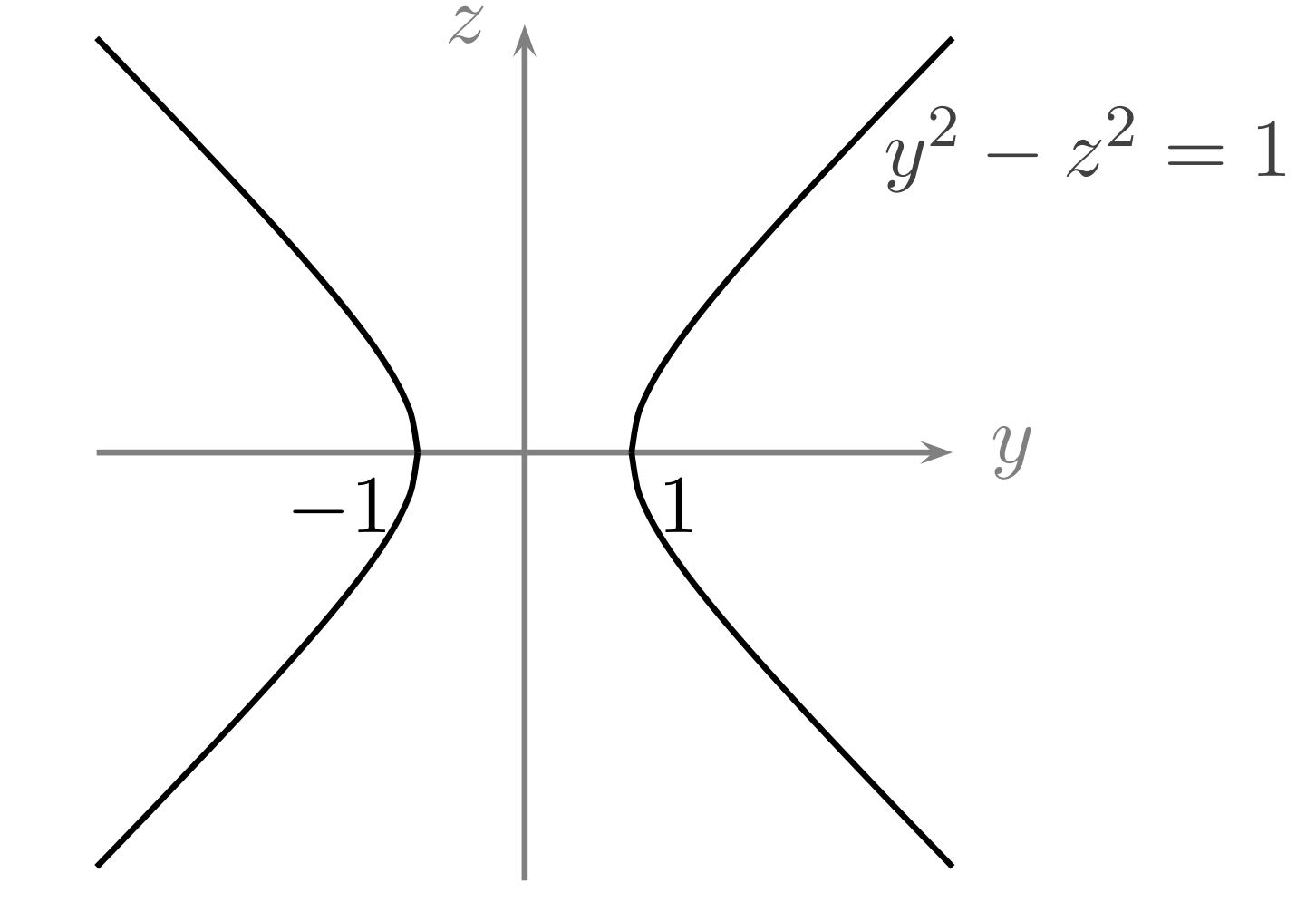
For the profiles, if x=0 you get y2−z2=1, which is a hyperbola:
Combining this, you get a hyperboloid of one sheet
Example. Sketch some level curves and profiles for the surface z=x2−y2, and hence describe the surface.
The level curves are of the form x2−y2=C:
If C=0, then y2=x2, i.e. the pair of straight lines y=x and y=−x.
If C>0, the level curves are hyperbolas opening left-and-right, crossing the x-axis at x=±C.
If C<0, the level curves are hyperbolas opening up-and-down, crossing the y-axis at y=±−C.
For the profiles, setting y=0 gives z=x2 (an upward parabola on the xz-plane), whilst setting x=0 gives z=−y2 (a downward parabola on the yz-plane). So the surface rises in the x-direction but falls in the y-direction; this is a saddle (formally, a hyperbolic paraboloid). Notice how the two profiles are genuinely different here, so unlike the paraboloid you actually need both of them.
The surface z=xy is the same saddle shape rotated 45∘ (rotating z=x2−y2 by 45∘ gives exactly z=2xy, so z=xy is that saddle rotated and vertically scaled by 21); its level curves xy=C are hyperbolas with the x- and y-axes as asymptotes, and along the line y=x the profile is the upward parabola z=x2 whilst along y=−x it is the downward parabola z=−x2.
Example. The surfaces z=x2+y2 and z=x2+y2 both have circles as their level curves. Explain how a sketch can still tell them apart.
For the paraboloid z=x2+y2, the level curve at height C is a circle of radius C, so the radii for C=1,2,3,4 are
1,2,3,2;
the circles bunch closer and closer together, meaning the surface gets steeper as you move outwards. For z=x2+y2, the level curve at height C is a circle of radius exactly C, so the radii are 1,2,3,4; evenly spaced circles, meaning constant steepness. The profiles confirm this: setting x=0 gives z=y2 for the first surface but z=∣y∣ (a V shape) for the second, so the second surface is a cone with a sharp tip at the origin. Two different surfaces can have identical-looking level curves; the spacing of the level curves and the profiles are what actually pin the surface down.
To introduce the notion of a partial derivative, consider the function F given by
F(x,y)=x2+y2.
The goal is to quantify the rate of change of F(x,y) at the point (1,2).
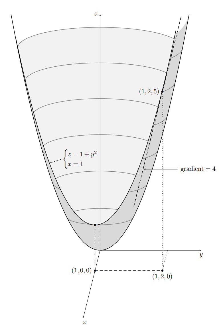
Since there are two variables, there are two places where the rate of change is changing: the x- and the y-direction. This means we can differentiate with respect to one of the variables while holding the other variables fixed. Since we are considering (1,2), we have x=1 and
z=F(x,y)=F(1,y)=1+y2,
since x is constant but y is not. This can also be thought of as the plane x=1 intersecting with the plot of F(x,y). The gradient in the y-direction can be calculated in the usual way:
gradient =dyd(1+y2)y=2=2yy=2=4.
Thus the rate of change of F(x,y) at (1,2) in the y-direction is 4.
A faster way of doing this is simply just treating x as a constant:
Fy(x,y)=2y
and then evaluating
Fy(1,2)=2×2=4.
The function Fy is called the partial derivative of F with respect to y.
Using the same method you can find Fx(1,2) and obtain 2.
The partial derivatives of a function F may be defined formally by using limits.
Note
The partial derivatives of F with respect to x and y are defined by
Fx(x,y)=h→0limhF(x+h,y)−F(x,y)
and
Fy(x,y)=h→0limhF(x,y+h)−F(x,y)
wherever these limits exist.
Example. Using the limit definition, find Fx where F(x,y)=x2y.
This agrees with the fast method of just treating y as a constant and differentiating with respect to x.
Example. Let F(x,y)=x2+y2 (the cone from 1.1). Show that Fx(0,0) does not exist.
Blindly differentiating gives Fx=x2+y2x, which is 00 at the origin, so we fall back to the limit definition:
which is 1 from the right but −1 from the left, so the limit does not exist. This makes sense geometrically; the cone has a sharp tip at the origin, so there is no well defined slope there (and, looking ahead to 1.3, no tangent plane either). If a question asks about a partial derivative at a point where the usual differentiation rules break down, use the limit definition.
Notation: Regarding Fx and Fy, they can also be denoted by
∂x∂F or D1F,
for Fx, while Fy may be denoted by
∂y∂F or D2F.
It is important to note that the notation involving the 'curly d' is a bit ambiguous. The notation D1F(y,x) simply means differentiate the first variable in the parenthesis and then evaluate the derivative at the point (y,x). To do the same with the 'curly d', one would write ∂x∂F(y,x). Here the x represents the first variable of the function whilst the x in parenthesis represents the second ordinate of the point (y,x).
Geometrical interpretations
∂x∂F is the slope of the surface z=F(x,y) in the x direction.
Fx(a,b) is the gradient of the tangent to the cross section at (a,b) when the surface z=F(x,y) is intersected with the plane y=b.
Similar definitions for ∂y∂F and Fy(a,b).
Example. Suppose that F(x,y)=3exy3siny. Find ∂x∂F and ∂y∂F.
For ∂x∂F, we treat y as a constant to yield
3y3exy3siny.
For ∂y∂F, we treat x as a constant and use the product rule to yield
Notation p2:
For second order partial derivatives, the notation is as follows:
∂x2∂2F∂y2∂2F∂x∂y∂2F∂y∂x∂2F means ∂x∂F(∂x∂F); means ∂y∂F(∂y∂F); means ∂x∂F(∂y∂F); means ∂y∂F(∂x∂F).
Note
The mixed derivative theorem Suppose that F is a function of two variables. If F and all its first and second order partial derivatives are continuous then
∂x∂y∂2F=∂y∂x∂2F
Since the definition of continuous is sort of ambiguous for two variables, a simple way to determine if it's continuous is simply to see if it's made up of many compositions of single variable functions. This means for a function F(x,y)=3xy4+exsiny, you can rewrite as F(x,y)=f(x)g(y)+h(x)k(y).
Most functions of two variables given in this course are continuous on their domains.
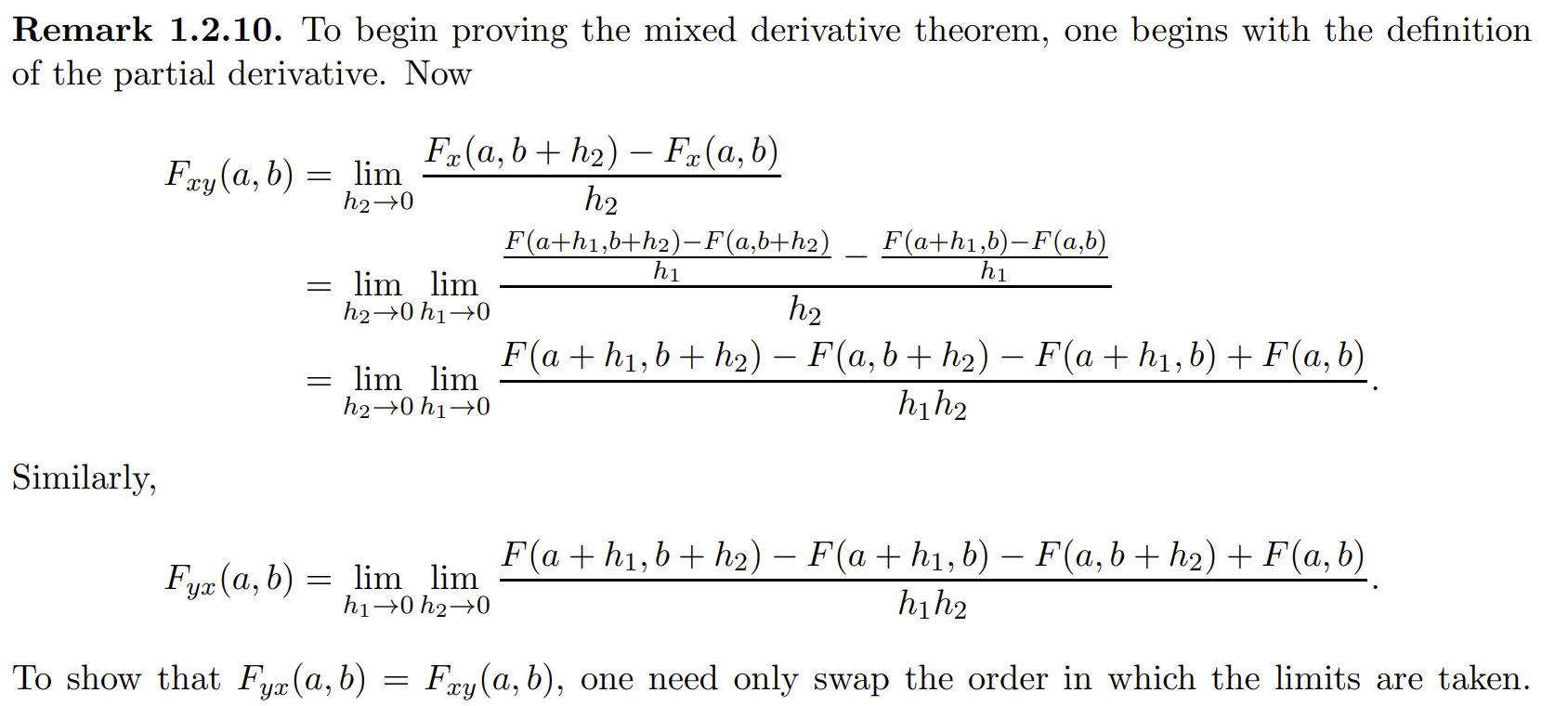
To prove the theorem, you use the definition of the partial derivative.
Example. Compute all second order partial derivatives of F, where F(x,y)=3xy4+exsiny, and verify the mixed derivative theorem.
The first order partial derivatives are
The two mixed partial derivatives are equal, exactly as the theorem promised; recall from earlier that this F is continuous since it is built from single variable continuous functions.
Example. Suppose that F(x,y)=x3y2+esinytan−1y. Find ∂x∂y∂2F.
Following the notation literally, we would have to differentiate with respect to y first; but ∂y∂F requires a product rule on esinytan−1y, which is horrible. Instead, notice that F and all its partial derivatives are continuous (compositions of single variable functions again), so the mixed derivative theorem lets us swap the order for free:
∂x∂F∂y∂x∂2F=3x2y2(the ugly term has no x, so it dies),=6x2y.
Therefore ∂x∂y∂2F=6x2y as well. When one order of differentiation is much messier than the other, check continuity and then use the mixed derivative theorem to pick the easy order.
A tangent plane is just like a tangent line in R2, but for surfaces in R3. While deriving an equation for the tangent plane, a formula for the normal vector to the surface at a given point is also obtained.
Example. Suppose that F(x,y)=x2+y2. Find the Cartesian equation of the tangent plane to the surface z=F(x,y) at the point where (x,y,z)=(1,2,5). Find also a vector n that is normal to the surface at this point.
First, intersect the surface z=x2+y2 with the plane x=1 to get
{z=1+y2x=1.
The gradient is Fy(1,2)=4. Using the point-gradient formula (y−y1)=m(x−x1) but for z=1+y2, a Cartesian equation for this tangent is given by
z−5=4(y−2),x=1.
If y=λ+2, then the equation of the tangent line in parametric form is
xyz=125+λ014
whenever λ∈R.
Similarly, we intersect the surface with the plane y=2 and repeat the previous steps to obtain
{z=4+x2y=2.
If x=μ+1 then the parametric vector form is
xyz=125+μ102
whenever μ∈R.
Since the two direction vectors lie in the tangent plane and the vectors are nonparallel, the tangent plane to the surface (1,2,5) is given by
xyz=125+λ014+μ102.
We can now convert the parametric vector form to a point-normal form, where the normal vector is given by the cross product of the two directions,
n=014×102=24−1.
Finally, you get the dot product of the normal and the coordinate vectors,
24−1⋅x−1y−2z−5=0.
By expanding the dot product, one obtains z=5+2(x−1)+4(y−2), which simplifies to
2x+4y−z=5.
This is the cartesian form of the tangent plane.
Notice how Fx(1,2)=2 and Fy(1,2)=4; each number being the coefficient of the cartesian equation respectively as well as components of the normal vector. This is not an accident;
Note
Proposition Suppose that F is a function of two variables and (x0,y0,z0) is a point that lies on the surface z=F(x,y). If the surface has a tangent plane at the point (x0,y0,z0), then the tangent plane is given by the equation
z=z0+Fx(x0,y0)(x−x0)+Fy(x0,y0)(y−y0)
and the normal vector to the surface at (x0,y0,z0) is given by
Fx(x0,y0)Fy(x0,y0)−1
Example. Find a normal vector n and the Cartesian equation of the tangent plane to the surface z=4x2y at the point (2,−1,−16).
The partial derivatives are
Fx(x,y)Fy(x,y)=8xy,=4x2,
so at the point (2,−1),
Fx(2,−1)Fy(2,−1)=8(2)(−1)=−16,=4(2)2=16.
By the proposition, a normal vector is
n=−1616−1
and the tangent plane is
z=−16−16(x−2)+16(y+1)=32−16x+16y.
Therefore the tangent plane is 16x−16y+z=32. Notice how much faster this is than the four-step vector geometry method; for a surface given explicitly as z=F(x,y), jump straight to the proposition.
Another way to find the normal vector is as follows;
if a surface is given in the form of g(x,y,z)=0, then the vector n=gxgygz evaluated at some point P on the surface, is a vector normal to the surface at P.
Example. Find the equation of the tangent plane to the ellipsoid 4x2+2y2+8z2=1 at the point P(0,1,2).
To find Fx(x,y), we use implicit differentiation and treat z as a function of x.
A vector normal to the ellipsoid at P can be derived by two methods, either from the method described in the earlier proposition or the gradient-vector method.
Using the gradient vector method we obtain,
n1=2xy4zP=011/2.
Using the proposition,
n2=−22⋅0−24⋅1−1=0−2−1
Notice that n2=−2n1; demonstrating that both methods are valid.
Hence, the equation of the tangent has the form
0x+1y+21z=d
for some constant d. Substituting P, the desired equation is 2y+z=4.
Example. Find the equation of the tangent plane to the sphere x2+y2+z2=1 at the point P(31,21,623).
First a quick sanity check that P actually lies on the sphere: 91+41+3623=364+9+23=1.
We could rearrange for z=1−x2−y2 and use the proposition, but the square root makes the partial derivatives messy; the gradient-vector method is much cleaner here. Writing g(x,y,z)=x2+y2+z2−1,
n=gxgygzP=2x2y2zP=2/3123/3.
Scaling by 3 to clear the fractions, we may instead use n=(2,3,23)T. The tangent plane then has the form
2x+3y+23z=d,
and substituting P,
d=32+23+623=64+9+23=6.
Therefore the tangent plane is 2x+3y+23z=6. If the surface is given implicitly, do not bother rearranging for z; use n=(gx,gy,gz)T directly.
Example. Find all points on the saddle z=x2−y2 where the tangent plane is horizontal.
A horizontal plane has normal vector (0,0,−1)T (up to scaling), so both partial derivatives must vanish:
Fx(x,y)Fy(x,y)=2x=0,=−2y=0,
which forces (x,y)=(0,0). So the only such point is the origin, where the tangent plane is z=0. Notice however that the plane z=0 intersects the surface along the level curves y=±x, so the tangent plane actually passes through the surface. A horizontal tangent plane does not mean the point is a maximum or a minimum; here it is a saddle point.
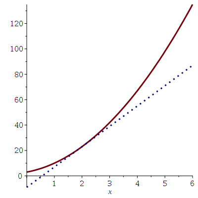
Evaluating ℓ(1.9)=21.4 whilst p(1.9)=21.43. Therefore, it is clear that the tangent line for a point x0 can be used to evaluate p(x1), where x1≈x0.
The image above depicts p(x) in red and the tangent ℓ(x) in blue.
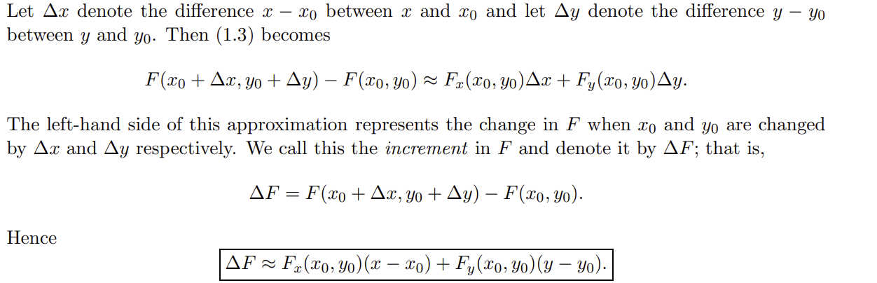
Rewriting Δx=x−x0 and Δf=f(x)−f(x0), we have
Δf≈f′(x0)Δx.
This is called differential approximation to Δf. Extending this to functions with two variables,
suppose that a surface given by z=F(x,y) has a tangent plane at the point (x0,y0,z0). The equation of the tangent is given by
z=z0+Fx(x0,y0)(x−x0)+Fy(x0,y0)(y−y0).
If (x,y) are near (x0,y0), and rewriting z0=F(x0,y0),
There's alot of iterating afterwards with Δ (image attached)
This formula is called the total differential approximation to ΔF. By suppressing the point of evaluation, the total differential approximation may be written as
ΔF≈∂x∂FΔx+∂y∂FΔy.
The approximation improves as Δx and Δy get smaller.
Example. Consider the paraboloid z=F(x,y)=52x2+32y2 at the point [5,1,10/9]. Find the total differential approximation of z=F(x,y) at [5.1,1.1] and compare it to F(5.1,1.1).
And Fy(5,1)=92.
Since they asked for the approximation for z and not just the change, you would use z=z0+Fx(x0,y0)(x−x0)+Fy(x0,y0)(y−y0).
Plugging in x0=5,y0=1,z0=910,
z=910+52(x−5)+92(y−1).
After simplifying,
z=52x+92y−910.
This is the equation for our tangent plane; plugging in (5.1,1.1) we get 1.173, whilst F(5.1,1.1) is 1.175.
Example. The ideal gas law asserts that the pressure P, volume V and temperature T of an ideal gas are related by the formula,
PV=kT,
where k is a constant. If the temperature increased by 4% and the volume is decreased by 5%, estimate the percentage increase in pressure.
Doing this the immediate way, which is simply plugging in V=0.95V and T=1.04T yields P=0.951.04VkT≈1.0947P,ΔP≈0.0947P, however, the question asks us to estimate, meaning we have to use the total differential approximation. Since we are calculating change, we use
ΔF≈∂x∂FΔx+∂y∂FΔy.
Rewriting,
P(T,V)ΔP≈∂T∂PΔT=VkT,+∂V∂PΔV.
Since we know that ΔT=0.04T and ΔV=−0.05V, we simply calculate ∂T∂P and ∂V∂P;
Notice how the 9% we obtained from the estimation is close to the exact answer of 9.47%.
NOTE: Another way to calculate z or find the linear approximation is to simply calculate ΔF and add it onto the original F value, this might be a bit easier.
Example. Use the total differential approximation of f(x,y)=x2+y2 to estimate 2.982+4.032.
Pick the nearby nice point (x0,y0)=(3,4), so that f(3,4)=9+16=5 and
ΔxΔy=2.98−3=−0.02,=4.03−4=0.03.
The partial derivatives are
fx(x,y)fy(x,y)=x2+y2x,=x2+y2y,
so fx(3,4)=53 and fy(3,4)=54. Then
Δf≈53×(−0.02)+54×0.03=−0.012+0.024=0.012.
Adding this onto the original value (as per the note above),
2.982+4.032≈5+0.012=5.012.
A calculator gives 5.012115, so the approximation is accurate to three decimal places. The whole trick with these 'estimate without a calculator' questions is choosing a nearby point where everything is clean.
No tools have absolute certainty in measurements; there is always a deviation from the exact value (i.e. a ruler can be off by ±0.1mm). Given this deviation, it is possible to use the total differential approximation to calculate how the maximum value of this deviation from the exact result. Given a function F(x,y), one can interpret ΔF as the error in the output given errors Δx and Δy. Typically, we don't know precise value of the deviation, but we can use bounds for the absolute errors ∣Δx∣ and ∣Δy∣.
Example. The dimensions of a cylinder are measured to the nearest millimeter using a measuring tape. The circumference is measured to be 22.0 cm and height is measured to be 15.0 cm. Use these measurements to (a) estimate the volume of the cylinder, and (b) estimate an upper bound for the percentage error in your answer to part (a).
(a). Since C=2πr,
V=πr2h=π(2πC2)h=4πC2h
By using C=22 and h=15,
V=π1815.
And so the volume is estimated to be π1815cm3, which is ≈577.75cm3. It says estimate in the question here only because the measuring tools were also estimated values, hence we "estimate" the final result; we don't use linear approx here.
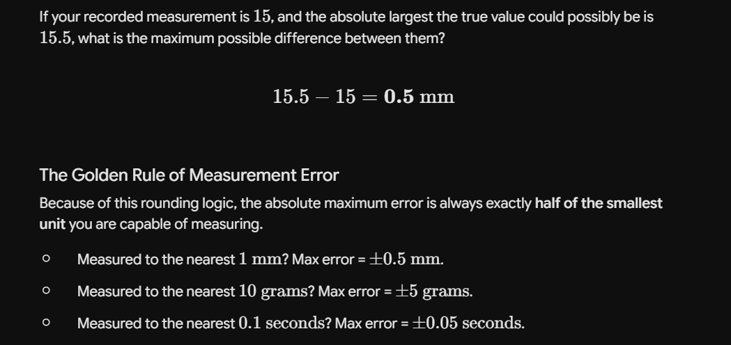
(b). Notice how the question says nearest millimeter, meaning ±0.5mm, or 0.05cm. The 0.5mm is for reasons below ig:
We convert to cm to match the units of the given inputs and make our lives easier.
Since both the circumference and height were measured, we can say that
So the upper bound for the absolute error in V is approximately 20π286 (or about 4.55cm3). To get the percentage error, we can do
Vmax∣ΔV∣×100%≈20π286⋅1815π×100%=3326%.
Hence the percentage error is no more than about 0.79%.
Example. The volume of a football in the shape of an ellipsoid of revolution with semi-axes of length a, b and b is given by
V=34πab2.
The values of a and b are measured to be 12.0 cm and 7.0 cm respectively, each to the nearest millimetre. (a) Calculate the volume of the football, (b) estimate the maximum absolute error in the calculated value of V, and (c) hence estimate the percentage error.
(a) Substituting the measurements,
V=34π(12)(7)2=784π≈2463 cm3.
(b) Measuring to the nearest millimetre again means ∣Δa∣≤0.05 and ∣Δb∣≤0.05 (converted to cm). The partial derivatives evaluated at (a,b)=(12,7) are
Therefore the volume is 784π cm3 with a percentage error of no more than about 1.85%. Notice how the error in b contributes over three times as much as the error in a, since b appears squared in the formula.
Example. The specific gravity S of a solid is given by
S=A−WA,
where A and W are its weights in air and water respectively. If A and W are measured to be 15.1 g and 5.1 g respectively, and each measurement has an error whose absolute value is at most 0.2 g, estimate the maximum error in the calculated value of S.
Differentiating with respect to A (holding W constant) using the quotient rule,
Hence the maximum error in S is approximately 0.0404. Do not plug ΔA=ΔW=0.2 straight into the total differential approximation; the negative coefficient would make the errors partially cancel and give 0.02, which underestimates the worst case. The worst case happens when the two measurement errors have opposite signs, which is exactly why the absolute values are essential.
Suppose we have V(h,r)=πr2h. If we wanted a linear approximation of V, we would usually find Vh, Vr, and do ΔV=VhΔh+VrΔr;
ΔV=(πr2)Δh+(2πrh)Δr,
this gets us the absolute error, if we want the fractional error we simply divide by V to understand the weight of each error:
VΔVVΔV=πr2h(πr2)Δh+πr2h(2πrh)Δr=hΔh+2rΔr.
Since Δr has a coefficient of 2, it means that an error on r has more weighting than an error on h. This makes sense as the original equation for V has r2 meaning it is more dominant compared to just h.
But doing all that working out is very tedious, we have to take two derivatives, divide by V and do lots of algebra. This is where logarithms come in. If we take the natural log (ln) of both sides,
lnVlnV=ln(πr2h)=lnπ+2lnr+lnh
and then take the differential of every single piece, remembering that the derivative of ln(x) is simply xdx,
VΔV=0+2rΔr+hΔh.
This immediately gives us the same result as before with minimal lines of working out.
Example. A triangle has two sides of length a and b with an included angle measuring 3π radians. Given that a increases by 5%, b decreases by 6% and the included angle increases by 2%, estimate the percentage increase of area of the triangle
(the constant ln21 differentiates to zero, so the working is otherwise unchanged)
here, each dx represents the relative change to x, so da=0.05a, meaning if we divide da by a, we only get the change in percentage. Therefore, we need to multiply dC by 3π since our angle, C, was given as 3π. Calculating, we get our area change to be ≈0.00209 or 0.209%.
Example. The specific volume v of a compressible fluid flowing through a section of area A with mean velocity V is given by
v=kAV,
where k is a constant. If v decreases by 5% and A increases by 4%, estimate the percentage change in V.
The unknown percentage this time is on the right hand side, but the log trick handles it the exact same way. Taking ln of both sides,
lnvvΔv=lnk+lnA+lnV=0+AΔA+VΔV.
Substituting vΔv=−0.05 and AΔA=0.04,
−0.05VΔV=0.04+VΔV=−0.09.
Therefore the velocity decreases by approximately 9%. Basically, once everything is written in terms of relative changes, you can rearrange for whichever percentage is missing; the log trick is not just for finding the error in the output.
Recall, the chain rule is simply used by calculating the derivative of f(g(x)) or g(f(x)).
If f and g are functions of one variable, then the derivative of f∘g may be calculated using the chain rule for functions of one variable:
dxdf(g(x))=f′(g(x)g′(x).
To calculate their partial derivatives, we use a chain rule for functions of more than one variable.
Suppose that F is a function of x and y and that x and y are each functions of t. A small change Δt in t produces a corresponding change Δx and Δy in x and y. These changes in turn produce a corresponding change ΔF in F. By the total differential approximation,
ΔF≈∂x∂FΔx+∂y∂FΔy
with the approximation getting better as Δx and Δy approach zero. If we divide through by Δt then
ΔtΔF≈∂x∂FΔtΔx+∂y∂FΔtΔy.
As Δt→0,
ΔtΔx=Δtx(t+Δt)−x(t)→dtdx
and
ΔtΔy=Δty(t+Δt)−y(t)→dtdy.
If we also view F as a function of t then, ΔtΔF→dtdF. So then the total differential approximation becomes
dtdF=∂x∂Fdtdx+∂y∂Fdtdy.
The above chain rule has many ambiguities. Firstly, the F on the LHS is a function of one variable t being differentiated with respect to t, whilst the function on the RHS is a function of two variables x,y being evaluated at a correct point.
This can be better interpreted with the following example.
Suppose you have a function F(x,y) that depends on longitude (x) and latitude (y);
F(x,y)=x2+2y2,
with the longitude and latitude defined as
x(t)=3t,y(t)=2t.
What is the rate of change for F at t=1?
Using the chain rule,
∂x∂F=2xdtdx=3,∂y∂F=4y,dtdy=2.
Putting them together,
dtdF=∂x∂Fdtdx+∂y∂Fdtdy=3×2x+2×4y,
since x(1)=3 and y(1)=2,
dtdF=(3×2×3)+(2×4×2)=18+16=34.
Therefore the rate of change is 34 km/h.
However, this is wrong as F is being treated as both as F(x,y) and F(t);
we can create a brand new function g(t) instead and plug in x(t)=3t, y(t)=2t directly,
g(t)=(3t)2+2(2t)2=9t2+8t2=17t2.
Because this is now a 1D function, we can just take the normal derivative,
g′(t)g′(1)=34t=34(1)=34 km/h.
The chain rule is usually much faster for complex problems however, but the point of this is to show that technically the notation for the chain rule is illegal.
We can express this chain rule without these ambiguities.
Note
Theorem
*Suppose F is a function of two variables and that x and y are both functions of one variable. Define the function ϕ by ϕ(t)=F(x(t),y(t)) and the point (x0,y0) by (x0,y0)=(x(t0),y(t0)). The derivative of ϕ at a point to can be defined as
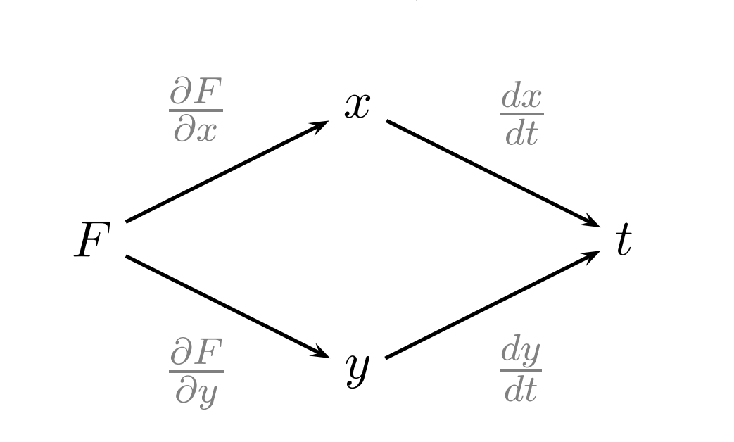
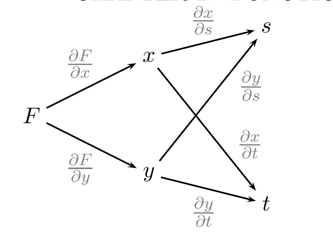
This formula and the one mentioned prior are equivalent, the former is easier to remember whilst the latter is more precise. You can use the chain diagram to memorise the rule.
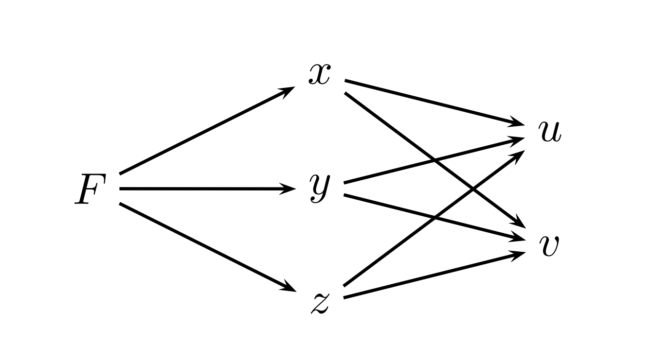
To construct the diagram, draw an arrow from each function to each of its variables. Then dtdF is the sum of all paths (left to right) from F to t, where the derivatives are multiplied across each path.
Example. The kinetic energy of a object with mass m (kilograms) and velocity v (metres per second) is given by
K=21mv2.
Suppose you drop an orange, where
the orange has a mass of m=65 kilograms,
the acceleration due to gravity is dtdv=−9.8 m/s2.
Find dtdK and hence dtdK∣v=2.
By the chain rule, the kinetic energy with respect to time is:
Here, v0 is 2, hence the answer is −49/3. Notice how m is not a function of t whilst v is, so the side of the equation using m just turns into 0.
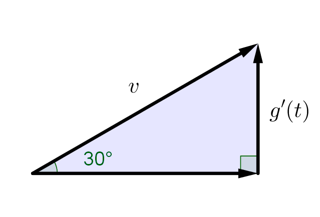
It is not actually necessary to know an explicit formula for the functions f and g, only their derivatives are required. Example. Suppose you drive a car up a steep mountain road at a constant speed of v=10 km/h. The gradient of the mountain is 30 degrees. If g(t) represents the altitude (in km) of the car at time t (in hours) then, what is the rate of change in altitude?
Furthermore, let f(h) represent the temperature at h kilometers above sea level. The temperature drops at a constant rate of 13/2 degrees for every kilometer above sea level. Find f′(h).
The composite function f(g(t)) represents the temperature at time t. By the chain rule the temperature changes with time at a rate of dtdf(g(t))=f′(g(t))g′(t). Find dtdf(g(t)).
To solve this, we can just use basic trigonometry to find the rate of change for the altitude:
We are given that the temperature drops at a constant rate of 13/2 degrees per kilometer, so f′(h)=−13/2.
Finally, calculating the composite rate of change:
dtdf(g(t))=f′(g(t))g′(t)=−213×5=−32.5 degrees per hour.
It might seem confusing to jump back to standard Calculus 1 formulas (like f′(g(t))g′(t)) after just learning the multivariable dependency trees. But they are actually the exact same formula.
If we draw the dependency tree for this car ride:
Top (Final Output): Temperature (T)
Middle (Middleman): Altitude (h)
Bottom (Foundation): Time (t)
Because Temperature only depends on Altitude, and Altitude only depends on Time, our tree doesn't branch. It is just a single, straight stick: T→h→t.
Since there are no "split loyalties" (multiple variables at the same level), we don't need the curly partial derivative symbol (∂). It straightens out into a standard total derivative (d):
dtdT=dhdTdtdh
This perfectly matches our calculation above: dhdT is f′(h) and dtdh is g′(t).
The chain rule also gives a very slick way of doing implicit differentiation. Suppose a curve in R2 is given implicitly by F(x,y)=0, and we view y as a function of x along the curve. Then F(x,y(x))=0 for all x, and differentiating both sides with respect to x using the chain rule (here the parameter t is just x itself, so dxdx=1),
∂x∂Fdxdx+∂y∂FdxdyFx+Fydxdy=0=0.
Rearranging,
dxdy=−FyFx,
provided Fy=0.
Example. Find the gradient of the curve x3+y3=6xy at the point (3,3).
First check the point is on the curve: 27+27=54=6×3×3. Now let F(x,y)=x3+y3−6xy, so the curve is F(x,y)=0. Then
Fx(x,y)Fy(x,y)=3x2−6y,=3y2−6x,
and so
dxdy=−Fy(3,3)Fx(3,3)=−27−1827−18=−1.
Therefore the gradient of the curve at (3,3) is −1. In MATH1131 you would differentiate the whole equation term by term and painfully collect all the dxdy terms; the boxed formula does all of that in one line. It is also worth remembering that the formula fails wherever Fy=0; those are the points where the curve has a vertical tangent.
We now examine the case when F is a function of x,y, where each x,y is a function of both s and t:
F=F(x,y),x=x(s,t) and y=y(s,t).
If we treat s as a constant and differentiate F with respect to t, the chain rule gives
∂t∂F=∂x∂F∂t∂x+∂y∂F∂t∂y.
Similarly, if we treat t as a constant and differentiate F with respect to s, then the chain rule gives
∂s∂F=∂x∂F∂s∂x+∂y∂F∂s∂y.
You can use the chain diagram to remember the chain rules.
Example. Suppose that z=F(x,y). Express the point (x,y) in terms of polar coordinates (r,θ). Hence express ∂r∂z and ∂θ∂z in terms of x,y,Fx and Fy. Finally, show that partial derivatives satisfy the equation
r∂r∂z+∂θ∂z=(x−y)∂x∂F+(x+y)∂y∂F.
Polar coordinates are simply just x=rcosθ and y=rsinθ, meaning r2=x2+y2, and we are givne z=F(x,y).
The chain rule gives
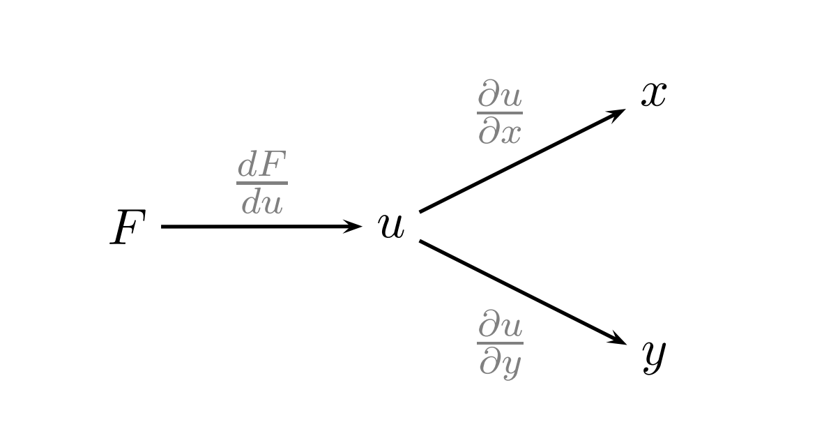
There is one more use case of the chain rule. Suppose F is a function of u and u is a function of x and y. This is written as
F=F(u) and u=u(x,y).
The chain rules are then,
∂x∂F=dudF∂x∂u
and
∂y∂F=dudF∂y∂u.
The chain diagram can be seen as follows:
Example. Suppose that f is a differentiable function of a single variable and F(x,y) is defined by F(x,y)=f(x2−y).
(a) Show that F satisfies the partial differential equation
∂x∂F+2x∂y∂F=0.
(b) Given that F(0,y)=siny for all y, find a formula for F(x,y).
(a) This is exactly the F=F(u), u=u(x,y) setup with u(x,y)=x2−y. The chain rules give
no matter what f actually is.
(b) Setting x=0 gives F(0,y)=f(−y)=siny. Substituting s=−y (so y=−s),
f(s)=sin(−s)=−sins.
Therefore
F(x,y)=−sin(x2−y)=sin(y−x2).
It is worth double checking: F(0,y)=siny, and Fx=−2xcos(y−x2) whilst Fy=cos(y−x2), so Fx+2xFy=0 as required. Questions like this look intimidating because f is never specified, but (just like the mountain road example earlier) only the derivative is ever needed; write everything in terms of f′(u) and watch it cancel.
It's sort of self-explanatory what this is abt.
Until now we have only discussed functions of two variables. In this section, the ideas met in this chapter are generalised to functions of three variables. We present a summary only.
Suppose that F is a function of three variables x, y and z. The partial derivatives of F are defined by
Fx(x,y,z)=h→0limhF(x+h,y,z)−F(x,y,z)
Fy(x,y,z)=h→0limhF(x,y+h,z)−F(x,y,z)
Fz(x,y,z)=h→0limhF(x,y,z+h)−F(x,y,z)
wherever these limits exist. Equivalent notation for each of these partial derivatives is given below:
Fx=∂x∂F=D1F,Fy=∂y∂F=D2F,andFz=∂z∂F=D3F.
If (a,b,c) is a point in R3 then Fx(a,b,c) is the rate of change of F in the x-direction at (a,b,c). Similarly, Fz(a,b,c) is the rate of change of F in the z-direction at (a,b,c).
The partial derivatives of F are calculated by differentiating F with respect to one variable and treating the other variables as constants. For example, if
Therefore dtdw=2t. We can sanity check by substituting first: w=cos2t+sin2t+t2=1+t2, whose derivative is indeed 2t. Geometrically, the point (x,y,z) spirals up a helix; the circular motion in x and y never changes the distance from the z-axis, so the only contribution to w comes from climbing in z. This is also a reminder that when x(t), y(t) and z(t) are explicitly known, substituting first is sometimes faster than the chain rule; the chain rule becomes essential when only the rates (and not the formulas) are given.
Example. The sides of a rectangular box are measured with percentage errors of at most 1%, 2% and 3% respectively. Estimate the maximum percentage error in the calculated volume.
The log trick from 1.4 generalises to three variables with zero extra effort. Since V=xyz,
lnVVΔV=lnx+lny+lnz=xΔx+yΔy+zΔz.
Taking absolute values and using the triangle inequality,
Therefore the percentage error in the volume is at most about 6%. Since each side appears to the first power, the percentage errors simply add; if the formula were, say, V=x2yz, the error in x would count twice.